17 Autoencoders
Reference: Ch.19 Bishop
One well-established approach to learning internal representations is the autoencoder architecture: a neural network having the same number of output units as inputs and which is trained to generate an output y that is close to the input x. Once trained, an internal layer within the neural network gives a representation z(x) for each new input. Such a network can be viewed as having two parts:
- Encoder: maps the input x into the hidden representation z(x)
- Decoder: maps z(x) onto the output y(z)
To find non-trivial solutions we can:
- Restrict the dimensionality of z relative to that of x
- Require z to have a sparse representation
- Modify the training process such that the network has to learn to undo corruptions to the input vectors
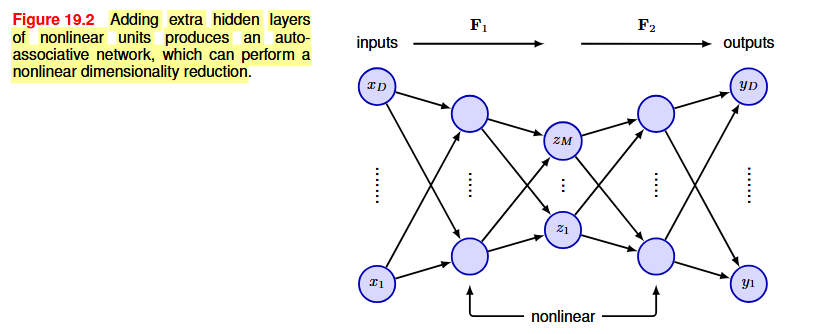
What we are gonna do is to make use of the nonlinearity of neural networks to define a form of nonlinear PC in which the latent manifold is no longer a linear subspace of the data space. This is done by optimizing the weights so as to minimize some measure of the reconstruction error between inputs and outputs. We use a sum-of-squares error of the form
E(w) = \dfrac{1}{2} \sum_{n = 1}^N ||y(x_n, w) - x_n||^2
If we use a simple multilayer perceptron with a hidden layer and an output layer, even with nonlinear units in the hidden layer, we will learn to span the same subspace as PCA: both PCA and neural networks rely on linear dimensionality reduction and minimize the same sum-of-squares error function. The situation is different when we add multiple nonlinear layers.
Instead of limiting the number of nodes in one of the hidden layers, an alternative way to constrain the internal representation is to use a regularizer to encourage a sparse representation, leading to a lower effective dimensionality. A simple choice is the L_1 regularizer since this encourages sparseness. This is called sparse autoencoder.
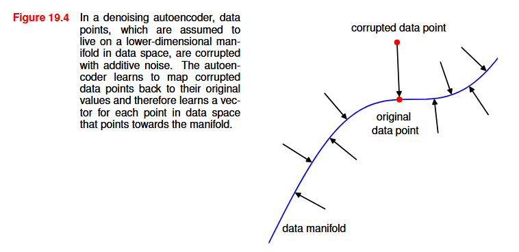
An alternative approach is to use a denoising autoencoder: the idea is to take each input vector x_n and to corrupt it with noise to give a modified vector \hat{x}_n which is then input to an autoencoder to give an output y(\hat{x}_n, w). The network is trained to reconstruct the original noise-free input vector by minimizing the sum-of-squares error applied to y(\hat{x}_n, w) instead of y(x_n, w).
By learning to denoise the input data, the network is forced to learn aspects of the structure of that data. The autoencoder learns to reverse the distortion vector \hat{x}_n - x_n and therefore learns a vector for each point in data space that points towards the manifold and therefore towards the region of high data density.
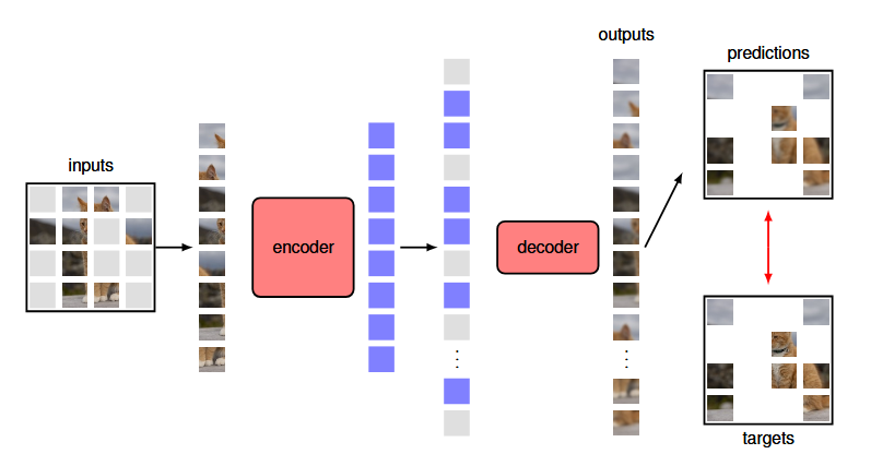
Another approach is to use a masked autoencoder: the process is the same of a denoising autoencoder, however in this case, the form of corruption is masking, or dropping out, part of the input. This technique is generally used in a vision transformer architecture: compared to language, images have much more redundancy along with strong local correlations. Omitting a single word from a sentence can greatly increase ambiguity whereas removing a random patch from an image typically has little impact. However, this kind of autoencoder works well even with texts and can be applied to any modality. The output of the decoder is followed by a learnable linear layer that maps the output representation into the space of pixel values, and the training error function is simply the mean squared error averaged over the missing patches for each image. After training, the decoder is discarded and the encoder is used to map images to an internal representation for use in downstream tasks.
17.1 Variational Autoencoders
The VAE is a generative model. Its primary goal is not just to reconstruct inputs, but to learn the underlying probability distribution of the data so it can generate new data.
17.1.1 How is it Different from a Standard Autoencoder?
| Feature | Standard Autoencoder (AE) | Variational Autoencoder (VAE) |
|---|---|---|
| Goal | Reconstruction & Dimensionality Reduction. | Generation of new data. |
| Latent Space | A single, deterministic vector (a point). The space can be disorganized. | A probability distribution (defined by a mean and variance). The space is smooth and continuous. |
17.1.2 Encoder
The encoder takes an input and, instead of outputting a single vector, it outputs the parameters of a probability distribution. Typically, this is a Gaussian distribution, so the encoder outputs two vectors:
- A mean vector (\mu)
- A log-variance vector (\log(\sigma^2))
These two vectors define a “cloud” of possible points in the latent space that could represent the input. Using log-variance is a technical trick for numerical stability during training.
We need to get a specific point z from the distribution our encoder just defined. The obvious way is to sample from it: z \sim \mathcal{N}(\mu, \sigma^2).
Problem: The sampling operation is random and has no clear gradient, so we can’t use backpropagation to train the encoder.
Solution: The Reparameterization Trick. We re-formulate the sampling process to make it trainable:
- Sample a random noise vector \epsilon from a simple, fixed distribution (usually the standard normal distribution N(0, 1)).
- Calculate the latent vector z as: z = \mu + \epsilon \cdot \sigma
Now, the network still produces a sample z from the desired distribution, but the random part (\epsilon) is external. The gradient can flow back through the \mu and \sigma vectors to the encoder, allowing it to be trained.
17.1.3 Decoder
The decoder works just like in a standard autoencoder: it takes a point z from the latent space and tries to reconstruct the original input image from it.
Because the latent space is continuous and smooth, if you take two points z_1 and z_2 and feed, for example, the midpoint \dfrac{z_1 + z_2}{2} into the decoder, you’ll get a plausible image that looks like a mix between the two points.
17.1.4 Training
The VAE is trained to optimize a special two-part loss function: Total Loss = Reconstruction Loss + Regularization Loss
- Reconstruction Loss: same as the standard autoencoder loss, it measures how different the decoder’s output is from the original input.
- Regularization Loss: this is the “variational” part. This loss measures how much the distribution produced by the encoder N(\mu, \sigma^2) differs from a standard normal distribution. It’s calculated using the Kullback-Leibler (KL) Divergence. This loss acts as a regularizer. It forces all the distributions that the encoder creates to stay close to the center of the latent space, because we are optimizing against a standard normal distribution. This has two effects:
- Continuity: It prevents the encoder from “cheating” by assigning each input its own spot in the latent space. It forces the “clouds” for different inputs to overlap, creating the smooth and continuous space.
- Generativity: Since all the encoded distributions are roughly centered around N(0, 1), we can later generate new samples by sampling a random point z from N(0, 1) and feeding it to the decoder.