3 Classification
References: Bishop 4, 4.1
The goal is to take an input vector x and to assign it to one of K discrete classes. In the most common scenario, the classes are disjoint, so that each input is assigned to one and only one class. The input space is divided into decision regions whose boundaries are called decision boundaries.
Here we consider linear models, by which we mean that the decision surfaces are linear functions of the input vector x and hence are defined by (D - 1)-dimension hyperplane within the D-dimensional input space. Datasets whose classes can be separated exactly by linear decision surfaces are said to be linearly separable.
How to represent the target values in order to represent class labels? For probabilistic models, the most convenient, in the case of two-class problems, is the binary representation in which there is a single target variable t \in \{0, 1\} such that t = 1 represent C_1 and t = 0 represents C_2. For K > 2 classes, we can use a 1-of-K coding scheme in which t is a vector of length K such that if the class is C_j, then all elements t_k of t are zero except for t_j, which is equal to 1.
We identify three approaches to the classification problem. The simplest involves constructing a discriminant function that directly assigns each input vector x to a specific class. A more powerful approach models the conditional probability distribution p(C_k | x) in an inference stage, and then subsequently uses this distribution to make optimal decisions. There are two different approaches to determining p(C_k | x). One technique is to model them directly, by representing them as parametric models and then optimizing the parameters using a training set. Alternatively, we can adopt a generative approach in which we model p(x | C_k), together with the prior probabilities p(C_k) for the classes, and then we compute p(C_k | x) using Bayes’ theorem (an example of this approach is the Naive Bayes model).
3.1 Linear Regression to do classification
For classification problems, we wish to predict discrete class labels, or more generally posterior probabilities that lie in (0, 1). To achieve this, we transform the linear function using a nonlinear function f(\cdot) called activation function
y(x) = f(w^Tx + w_0)
The decision surfaces correspond to y(x) = constant, and hence the decision surfaces are linear functions of x, even if the function f(\cdot) is nonlinear, so we still call it a linear model. However, they are no longer linear in the parameters due to the presence of f(\cdot). Obviously, if we apply basis functions we lose also the linearity on the input vector x.
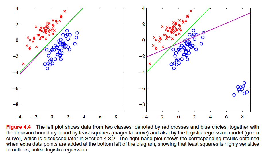
The least-squares approach gives an exact closed-form solution for their discriminant function parameters. However, even as a discriminant function is suffers from some problems: it lacks robustness to outliers, and the sum-of-squares error function penalizes predictions that are ‘too correct’ in that they lie a long way on the correct side of the decision boundary.
3.2 Discriminant Functions
A discriminant is a function that takes an input vector x and assigns it to one of K classes, denoted C_k.
3.2.1 Two classes
The simplest representation of a linear discriminant function is obtained by taking a linear function of the input vector x
y(x) = w^Tx + w_0
An input vector x is assigned to class C_1 if y(x) \geq 0 and to class C_2 otherwise. The corresponding decision boundary is therefore defined by the relation y(x) = 0, which corresponds to a (D - 1)-dimensional hyperplane within the D-dimensional input space. The vector w is orthogonal to every vector lying within the decision surface, and so w determines the orientation of the decision surface; w_0 determines the location of the decision surface.
3.2.2 Multiple classes
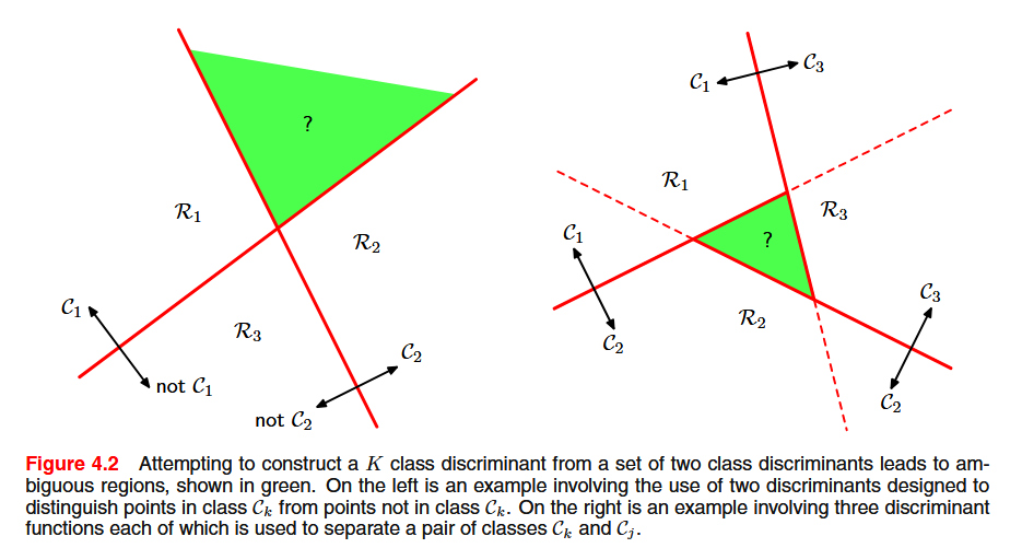
We have three approaches:
- One-versus-the-rest classifier: using K - 1 classifiers each of which solves a two-class problem of separating points in a particular class C_k from points not in that class
- One-versus-one classifier: using \frac{K(K-1)}{2} binary discriminant functions, one for every possible pair of classes. Each point is then classified according to a majority vote amongst the discriminant functions.
These two approaches suffer from the problem of ambiguous regions.
We can avoid this problem by considering a single K-class discriminant comprising K linear functions of the form
y_k(x) = w_k^Tx + w_{k0}
and then assigning a point x to class C_k if y_k(x) > y_j(x) for all j \neq k. The decision boundary between class C_k and class C_j is given by y_k(x) = y_j(x) and hence corresponds to a (D - 1)-dimensional hyperplane defined by
(w_k - w_j)^T x + (w_{k0} - w_{j0}) = 0
The decision regions of such a discriminant are always singly connected (without ‘holes’) and convex. If two points x_A and x_B both lie inside the same decision region R_k, then any point \hat{x} that lies on the line connecting these two points must also lie in R_k, and hence the decision region must be singly connected and convex.