9 Clustering
Clustering techniques perform unsupervised learning, the aim is to divide instances into natural groups.
Clusters can be:
- disjoint vs overlapping
- deterministic vs probabilistic
- flat vs hierarchical
The idea is to find clusters that have an high intra-cluster similarity and a low inter-cluster similarity.
9.1 K-means
- Choose K random cluster centers
- Assign each instance to closest cluster center (Euclidean distance/Hamming)
- Recompute cluster centers by computing the average (centroid) of the instances pertaining to each cluster
- If cluster centers have moved, go back to 2.
Another termination criterion is to stop when assignment of instances to cluster centers has not changed.
In this way, we determine a solution that achieves a local minimum of the distance, so result can vary significantly based on the initial choice of seeds. To increase the chance of finding global optimum we restart the procedure with different seeds.
Another problem is that k-means identifies only spherical-shaped clusters.
9.1.1 Bisecting k-means
To cope with the problem from which k-means suffers, we can adopt this algorithm:
- Start with a single cluster with all the points
- While the number of clusters < K
- Choose the cluster to be divided (the one with maximum internal variance or the bigger one)
- k-means(k=2)
- Replace the cluster with the two new subclusters
9.2 General improvements
To find the right number of clusters, we can try out different values of k and see which one minimizes the total squared distance of all points to their cluster center. However, this may not be feasible in practice and tends to favor clusters having just one instance. Alternatively, we can use the elbow method: the method consists of plotting the variation as a function of the number of clusters and picking the elbow of the curve as the number of clusters to use.
To cope with categorical features we adopt k-medoids rather than k-means: the medoid is the element that has the lowest dissimilarity with respect to the others.
To cope with new instances, there exists an incremental clustering approach called COBWEB.
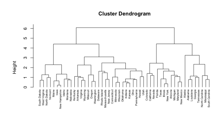
9.3 Hierarchical clustering
Bisecting k-means performs hierarchical clustering in a top-down manner (divisional clustering).
Standard hierarchical clustering performs clustering in a bottom-up manner (agglomerative clustering):
- Make each instance in the dataset into a trivial mini-cluster
- Find the two closest clusters and merge them; Repeat
- Clustering stops when all clusters are merged into a single cluster
To choose the two closest clusters we can choose one of these strategies:
- Single-linkage clustering: distance is measured by finding the two closest instances, one from each cluster, and taking their distance
- Complete-linkage: use the two most distant instances
- Average-linkage: take average distance between all instances
- Centroid-linkage: take distance of cluster centroids
- Group-average: take average distance in merged clusters
To cut the generated tree from the hierarchical algorithm and obtain a certain number of clusters we can use the following strategies:
Distance Threshold: select a distance threshold and cut the tree in a way that stops the merging of clusters when the distance between them exceeds that threshold.
Fixed Number of Clusters: decide in advance how many clusters you want and cut the tree at a level that results in exactly that number of clusters.
9.4 Evaluation
9.4.1 Internal Cluster Validation
Uses the internal information of the clustering process to evaluate the clustering structure without external information.
9.4.1.1 Silhouette Index
The silhouette value is a measure of how similar an object is to its own cluster compared to other clusters. The silhouette value ranges from -1 to +1, where a high value indicates that the object is well matched to its own cluster and poorly matched to neighboring clusters.
If most objects have a high value, then the clustering configuration is appropriate. If many points have a low or negative value, then the clustering configuration may have too many or too few clusters.
For data point i \in C_i, let a(i) = \dfrac{1}{|C_i| - 1} \cdot \sum_{j\in C_i, i\neq j} d(i, j) be the mean distance between i and all other data points in the same cluster, where |C_i| is the number of points belonging to cluster C_i, and d(i, j) is the distance between data points i and j in the cluster C_i (we divide by |C_i| - 1 because d(i, i) is not included in the sum).
a(i) is a measure of how well i is assigned to its cluster (the smaller the value, the better the assignment).
We then define the mean dissimilarity of point i to some cluster C_j as the mean of the distance from i to all points in C_j (where C_j \neq C_i).
For each data point i \in C_i, we now define
b(i) = \min_{j \neq i} \dfrac{1}{|C_j|} \cdot \sum_{j\in C_j} d(i, j)
to be the smallest mean distance of i to all points in any cluster to which i does not belong. The cluster with the smallest mean dissimilarity is said to be the “neighboring cluster” of i because it is its next best-fit cluster.
We now define a silhouette of one data point i as
s(i) = \begin{cases} \dfrac{b(i) - a(i)}{\max\{a(i), b(i)\}} & \text{if } |C_i| > 1 \\ 0 & \text{if } |C_i| = 1 \end{cases}
s(i) is bounded to the interval (-1, 1). a(i) is not clearly defined for clusters with size = 1, in which case we set s(i) = 0.
9.4.1.2 Dunn’s index
- For each cluster, compute the distance between each of the objects in the cluster and the objects in the other clusters
- Use the minimum of this pairwise distance as the inter-cluster separation
- For each cluster, compute the distance between the objects in the same cluster
- Use the maximal intra-cluster distance as the intra-cluster compactness
- Calculate the Dunn index as
D = \dfrac{\text{min.separation}}{\text{max.diameter}}
where min.separation is the minimum inter-cluster separation and max.diameter is the maximum intra-cluster compactness. Thus, Dunn index should be maximized.
9.4.2 External Cluster Validation
If we have a ground truth, we can compare the results measuring the agreement between clusters and ground truth.
9.4.3 Relative Cluster validation
Evaluates the clustering structure by varying different parameter values for the same algorithm. It is generally used for determining the optimal k (e.g. elbow method).
9.5 Probabilistic clustering
Instances have a certain probability of belonging to each cluster. The foundation for statistical clustering is the concept of mixture: a set of k probability distributions, representing k clusters, that govern the attribute values for members of that cluster.
A classic statistical clustering algorithm is the Expectation-Maximization algorithm:
- Expectation step: compute the cluster probabilities (the expected class values), that is, the probability of an example belonging to a certain cluster
- Maximization step: find the new parameters (mean, covariance) that maximize the function computed in the Expectation step.