5 KNN
5.1 Parametric vs Non-parametric models
- Parametric models assume a specific form for the distribution, that may turn out to be inappropriate for some application
- In Non-Parametric models the form of the distribution typically depends on the size of the dataset. They still contain parameters, but these control the model complexity rather than the form of the distribution.
5.1.1 Non-parametric models
They are typically simple methods to approximate discrete-valued or real-valued target functions, so they work for classification or regression problems.
The learning amounts to simply storing training data, and test instances are classified using similar training instances.
These models are defined following these assumptions:
- Output varies smoothly with input: points that are close to each other in the feature space are likely to have similar target values
- Data occupies sub-space of high-dimensional input space: local patterns can be exploited
- No strong distributional assumptions
5.1.2 The Nearest Neighbors approach
The idea is that the value of the target function for a new query is estimated from the known values of the nearest training examples.
To define what is near we need a similarity measure. A similarity measure d has the following properties:
- d(x, y) \geq 0, and d(x, y) = 0 \iff x = y
- d(x, y) = d(y, x)
If the triangular property is respected (d(x, y) \leq d(x, z) + d(z, y)), then we talk about a distance measure. A common distance measure is the Euclidean: ||x^a - x^b||_2 = \sqrt{\sum_{j = 1}^d (x_j^a - x_j^b)^2}
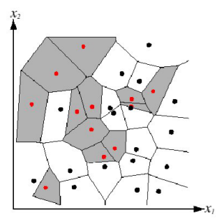
Nearest neighbor algorithm does not explicitly compute decision boundaries, but these can be inferred. We can use a visual tool called Voronoi diagram visualization that shows how the input space is divided into classes, and each line segment is equidistant between two points of opposite classes.
In order to avoid class noise we smooth the nearest neighbor algorithm by having k nearest neighbors vote. The first assumption allows us to think that this can mitigate this problem.
How do we choose k? We can use cross-validation, or, a rule of thumb is k < \sqrt{n}, where n is the number of “training” examples.
Another problem is that if some attributes of the input vector x have larger ranges, then they are treated as more important. The solution is to scale the range of each feature.
The last problem is given by the curse of dimensionality: irrelevant and/or correlated attributes add noise to distance measure, counteracting on the second assumption we made. The solution is to eliminate some attributes, or give a weight to attributes.
If we have features that are not numerical, we will need a distance that allows them to be compared, like the Hamming distance.
5.1.2.1 K-NN Algorithm
- Find k examples \{x^i, t^i\} closest to the test instance x
- Classification is done via majority class voting
5.1.2.2 Complexity Insight and Remedies
The complexity of the K-NN algorithm is \mathcal{O}(kdN), where d is the dimensionality, so it scales linearly with the number of examples. We can somehow mitigate it:
- Using a subset of dimensions
- Pre-sorting training examples into fast data structures like kd-trees, built picking a random dimension per level, finding the median value, splitting the data, and repeating that process. In this way we prune not promising paths when calculating the distance. The complexity becomes \mathcal{O}(dN) + \mathcal{O}(k), because in the worst case this can degenerate to a list.
- Computing an approximate distance like LSH (Locally-sensitive hashing), that divides data into l bucket (using hash functions) and computes the distance between buckets; the ratio is that due to the locality property similar points are more likely to end up in the same bucket.
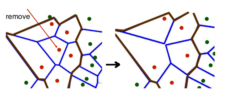
- Removing redundant data condensing them: if all Voronoi neighbors have the same class, then we can remove the point.