19 Neural NLP
19.1 Representing words as discrete symbols
The first challenge is to convert the words into a numerical representation that is suitable for use as the input to a deep neural network. One simple approach is to define a fixed dictionary of words and then use one-hot encoding. An obvious problem is that a realistic dictionary might have several hundred thousand entries, leading to vectors of very high dimensionality. Also, it does not capture any similarities or relationships. Both issues can be addressed by mapping the words into a lower-dimensional space through a process called word embedding in which each word is represented as a dense vector in a space of typically a few hundred dimensions.
19.1.1 word2vec
We can learn the matrix E from a corpus of text, and there are many approaches to doing this.
word2vec can be viewed as a simple two-layer neural network. A training set is constructed in which each sample is obtained by considering a ‘window’ of M adjacent words in the text. The samples are considered to be independent, and the error function is defined as the sum of the error functions for each sample.
There are two variants of this approach.
- Continuous bag of words (CBOW): the target variable for network training is the middle word, and the remaining context words form the inputs, so that the network is being trained to ‘fill in the blank’
- Skip-grams: reverses the inputs and outputs, so that the centre word is presented as the input and the target values are the context words
The intuition of skip-gram is:
- Treat the target word and a neighboring context word as positive examples
- Randomly sample other words to get negative examples
- Use logistic regression (hence the two-layer structure) to train a classifier to distinguish those two cases
- Use the learned weights as the embeddings
We want to train a classifier such that, given a tuple (w, c) of a target word w paired with a candidate context word c, it will return the probability that c is a real context word, P(+ | w,c).
The probability that word c is not a real context word for w is just P(- | w,c) = 1 - P(+ | w,c).
To find P we base it on the assumption that a word is likely to occur near the target if its embedding vector is similar (closer) to the target embedding. This means that two vectors are similar if they have a high dot product. To turn the dot product into a probability we use the sigmoid function.
P( + | w, c) = \sigma(c \cdot w) = \dfrac{1}{1 + \exp(-c \cdot w)} P(- | w, c) = 1 - P(+ | w,c) = \dfrac{1}{1 + \exp (c\cdot w)}
Skip-gram makes the simplifying assumption that all context words are independent, so
P(+ | w, c_{1:L}) = \prod_{i = 1}^L \sigma(c_i \cdot w) \log P(+ | w, c_{1:L}) = \sum_{i = 1}^L \log \sigma(c_i \cdot w)
The algorithm learns two embedding matrices: the target embeddings W and the context embeddings C, for a total of 2|V| vectors of dimension d. The final word representation is typically w_i + c_i, or simply w_i.
The loss function we will use to maximize the similarity of the target word, context word pairs drawn from the positive examples while minimizing the similarity of the (w, c_{neg}) pairs from the negative examples is the following
\begin{aligned} L &= -\log\left[P(+|w, c_{pos})\prod_{i=1}^{k}P(-|w, c_{neg_i})\right] \\ &= -\left[\log P(+|w, c_{pos}) + \sum_{i=1}^{k}\log P(-|w, c_{neg_i})\right] \\ &= -\left[\log P(+|w, c_{pos}) + \sum_{i=1}^{k}\log\left(1 - P(+|w, c_{neg_i})\right)\right] \\ &= -\left[\log\sigma(c_{pos}\cdot w) + \sum_{i=1}^{k}\log\sigma(-c_{neg_i}\cdot w)\right] \end{aligned}
19.1.2 FastText
Fasttext addresses a problem with word2vec: it has no good way to deal with unknown words. Fasttext deals with these problems by representing each word as a bag of n-grams, with special boundary symbols < and > added to each word. Then, a skipgram embedding is learned for each n-gram, and the word is represented by the sum of all of the embeddings of its constituent n-grams. Unknown words can then be represented by the sum of their constituent n-grams.
19.2 Attention
Transformers are based on the concept of the attention, which allows a network to give different weights to different inputs, with weighing coefficients that themselves depend on the input values. These models are known as transformers because they transform a set of vectors in some representation space into a corresponding set of vectors, having the same dimensionality, in some new space, that will have a richer internal representation: a transformer can be viewed as a richer form of embedding in which a given vector is mapped to a location that depends on the other vectors in the sequence.
The input data is a set of vectors \{x_n\} of dimensionality D. We will combine the data vectors into a matrix \mathbf{X} of dimensions N \times D (tokens \times features). The fundamental building block of a transformer is a function that takes a data matrix as input and creates a transformed matrix \hat{\mathbf{X}} of the same dimensionality as the output.
\hat{X} = \text{TransformerLayer}[\mathbf{X}]
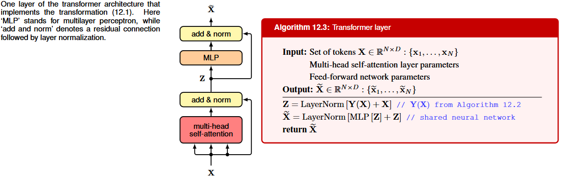
We can then apply multiple transformer layers in succession to construct deep networks. Each transformer layer contains its own weights and biases. A single transformer layer itself comprises two stages. The first stage implements the attention mechanism, which mixes together the corresponding features from different token vectors across the columns of the data matrix, whereas the second stage then acts on each row independently and transforms the features within each token vector.
19.2.1 Dot-product self-attention
We want to map the set of input tokens x_1, \ldots, x_N to another set y_1, \ldots, y_N having the same number of tokens, where the value of y_n should depend on all the vectors x_1, \ldots, x_N in the set. A simple way to achieve this is to define each output vector y_n to be a linear combination of the input vectors with attention weights a_{nm}:
y_n = \sum_{m = 1}^N a_{nm} x_m
If an output pays more attention to a particular input, this will be at the expense of paying less attention to the other inputs, and so we constrain the coefficients to sum to unity.
a_{nm} \geq 0, \qquad \sum_{m = 1}^N a_{nm} = 1
To compute these weights, we need to use a measure of similarity to work out how similar these input vectors are in order to understand the influence of x_n on the token represented by x_m. We can use the dot product passed through the softmax:
a_{nm} = \dfrac{\exp(x_n^T x_m)}{\sum_{m^{'} = 1}^N \exp(x_n^Tx_m^{'})}
In this case there is no probabilistic interpretation of the softmax function and it is simply being used to normalize the attention weights appropriately.
We can write this process into matrix notation XX^\mathrm{T} = \begin{bmatrix} x_1 \cdot x_1 & x_1 \cdot x_2 & \dots & x_1 \cdot x_N \\ x_2 \cdot x_1 & x_2 \cdot x_2 & \dots & x_2 \cdot x_N \\ \vdots & \vdots & \ddots & \vdots \\ x_N \cdot x_1 & x_N \cdot x_2 & \dots & x_N \cdot x_N \end{bmatrix} \text{Softmax}(XX^T) = \begin{bmatrix} a_{11} & a_{12} & \dots & a_{1n} \\ a_{21} & a_{22} & \dots & a_{2n} \\ \vdots & \vdots & \ddots & \vdots \\ a_{n1} & a_{n2} & \dots & a_{nn} \end{bmatrix} Y = \text{Softmax}(XX^T) X
This process is known as dot-product self-attention.
As it stands, the transformation is fixed, without the capacity to learn from data. Furthermore, each of the feature values plays an equal role in determining the attention coefficients; we would like the network to have the flexibility to focus more on some features than others. We can address both issues if we define modified feature vectors given by a linear transformation in the form
\hat{X} = XU
where U is a D \times D matrix of learnable weight parameters.
\mathbf{Y} = \text{Softmax}[XUU^TX^T]XU
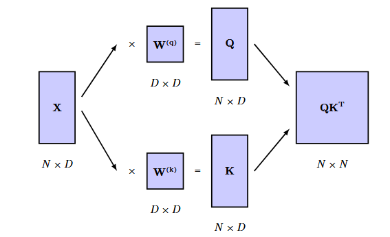
The problem is that the matrix XUU^TX^T is symmetric, while we want asymmetry: we might expect that a ‘hammer’ is strongly correlated with ‘tool’, whereas ‘tool’ should only be weakly associated with ‘hammer’ because there are many other kinds of tools besides hammers. We overcome these limitations by defining three matrices (query, key, value)
\mathbf{Q} = \mathbf{X}\mathbf{W}^{(q)}, \quad \mathbf{K} = \mathbf{X}\mathbf{W}^{(k)}, \quad \mathbf{V} = \mathbf{X}\mathbf{W}^{(v)}
W^{(k)} has dimensionality D \times D_k, where D_k is the length of x_n. Typically D_k = D W^{(q)} must have the same dimensionality D \times D_k so that we can form dot products between x_n and x_m.
W^{(v)} is a matrix of size D \times D_v, where D_v governs the dimensionality of the output vectors. To have the output representation of the same dimensionality of the input, D_v = D.
We can then generalize the first \mathbf{Y} we defined as
\mathbf{Y} = Softmax[QK^T]V
QK^T has dimension N \times N, \mathbf{Y} has dimension N \times D_v.
The idea behind these names is the following:
- We start from x_i, that is our query
- We compute the dot product (x_i, x_j) with each x_j to obtain a_{ij}, where x_j is our key
- The output is obtained with the linear combination, that is our value.
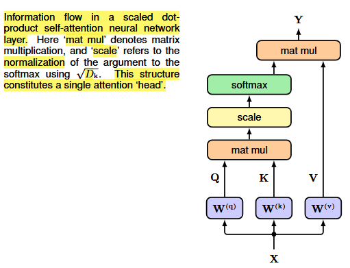
The gradients of the softmax become exponentially small for inputs of high magnitude, so in the final formula (scaled dot-product self-attention) we normalize the argument to the softmax using the standard deviation given by the square root of D_k.
\mathbf{Y} = \text{Attention}(\mathbf{Q}, \mathbf{K}, \mathbf{V}) = \text{Softmax} \left[ \dfrac{QK^T}{\sqrt{D_k}} \right] V
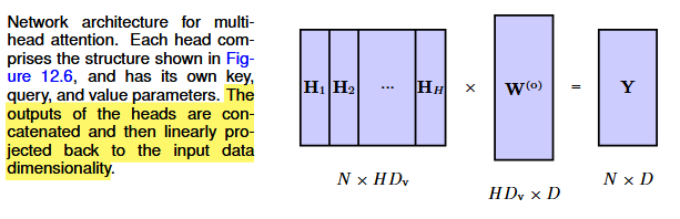
The attention layer described so far is called an attention head, and it captures data-dependent patterns of input vectors. We may want to capture multiple patterns of attention, instead of averaging over them. To do so, we use multiple attention heads in parallel. Simply, we have H heads with their own query, key, and value matrices. The heads are first concatenated into a single matrix, and the result is then linearly transformed using a matrix W^{(o)} to give a combined output in the form
\mathbf{Y}(\mathbf{X}) = \text{Concat}[H_1, ..., H_H] W^{(o)}
To improve training efficiency, we can introduce residual connections that bypass the multi-head structure. This is then followed by layer normalization
Z = LayerNorm[Y(X) + X]
Sometimes the layer normalization is replaced by pre-norm, in which the normalization layer is applied before the multi-head self-attention instead of after
Z = Y(X') + X, \text{where } X' = LayerNorm[X]
Attention mechanism, as shown in the first formula, is a linear conbination. Non-linearity does enter through the attention weights, and so the outputs will depend nonlinearly on the inputs via the softmax function, but the output vectors are still constrained to lie in the subspace spanned by the input vectors. We add non linearity using an MLP with D inputs and D outputs.
The query, key, and value matrices lack token order information, so we need to find a way to inject it into the network. To do so, we construct a position encoding vector r_n associated with each input position n, and we simply add the position vectors to the token vectors to give
\hat{x}_n = x_n + r_n
Residual connections preserve this positional information across layers. Common choices include sinusoidal functions of increasing wavelength (which generalize to unseen sequence lengths) and learned position encodings (which do not generalize beyond the training length).
19.3 Transformers
19.3.1 Decoder Transformers (GPT)
The goal is to use the transformer to construct an autoregressive model in which the conditional distributions p(x_n | x_1, \ldots, x_{n - 1}) are expressed using a transformer neural network that is learned from data. The model takes as input a sequence consisting of the first n - 1 tokens, and its corresponding output represents the conditional distribution for token n. If we draw a sample from this distribution then we have extended the sequence to n tokens and this new sequence can be fed back through the model to give a distribution over token n + 1, and so on.
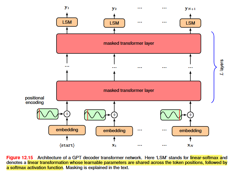
The architecture of a GPT model consists of a stack of transformer layers that take a sequence x_1, \ldots, x_N of tokens, each of dimensionality D, as input and produce a sequence \hat{x}_1, \ldots, \hat{x}_N of tokens, again of dimensionality D, as output. Each softmax output unit has an associated cross-entropy error function.
The model is trained in a self-supervised way: given a sequence x_1, \ldots, x_n, the target is the next token x_{n+1}. To gain efficiency, we process the entire sequence at once, so each token serves both as target for previous tokens and as input for following ones. To prevent the model from seeing future tokens:
- The input is shifted right by one step (input x_n → output y_{n+1}), with a special <start> token prepended.
- Masked attention is applied: pre-activation values for future positions are set to -\infty, so the softmax yields zero attention weights for later tokens.
At inference time, the model outputs a probability distribution over tokens via softmax; the chosen token is appended and the sequence is fed back to generate the next token, until an end-of-sequence token is produced.
19.3.2 Sampling strategies
We have already seen greedy decoding and beam search. An alternative is to use the top-k sampling: consider only the states having the top K probabilities and then sample from these according to their renormalized probabilities. A variant of this approach, called top-p sampling, calculates the cumulative probability of the top outputs until a threshold is reached and then samples from this restricted set of token states. A ‘softer’ version of top-K sampling is to introduce a parameter T called temperature into the definition of the softmax function
y_i = \dfrac{exp(a_i/T)}{\sum_j exp(a_j/T)}
- T = 0: greedy selection
- T = 1: normal softmax
- T \rightarrow \infty: the distribution becomes uniform across all states (hence, ‘more creativity’)
19.4 Encoder Transformer (BERT)
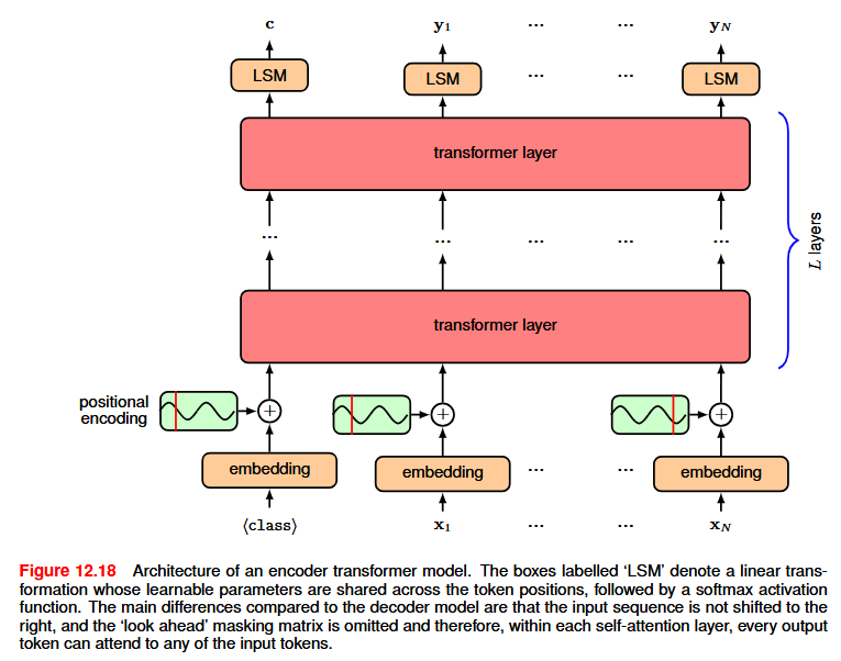
These are models that take sequences as input and produce fixed-length vectors. The first token of every input is a special <\text{class}> token. During pre-training, a random subset of tokens is replaced with <mask> and the model is trained to predict them — hence bidirectional, since the network sees context on both sides. Compared to decoders, encoders are less efficient (only masked tokens provide training signal) and cannot generate sequences. After pre-training, the encoder is fine-tuned by adding a task-specific output layer (e.g., a D \times K matrix for K-class classification, applied to the first output position).
19.4.1 Sequence-to-sequence transformers
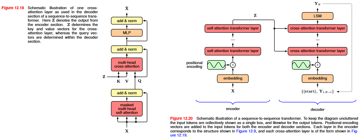
We use the translation from English to Dutch as an example. We can use a decoder model to generate the token sequence corresponding to the Dutch output, token by token, as discussed previously. The main difference is that this output needs to be conditioned on the entire input sequence corresponding to the English sentence. An encoder transformer can be used to map the input token sequence into a suitable internal representation, which we denote by Z. To incorporate Z into the generative process for the output sequence, we use a modified form of the attention mechanism called cross attention, that is, the self-attention except that although the query vectors come from the sequence being generated, in this case the Dutch output sequence, the key and value vectors come from the sequence represented by Z.
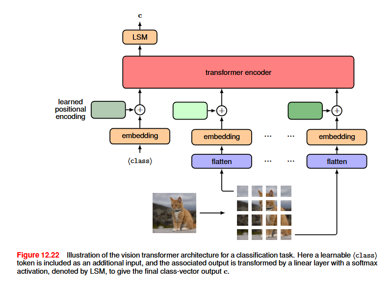
19.4.2 Vision Transformer
To feed images as tokens, each image is split into non-overlapping patches of size P \times P and then ‘flattened’ into a one-dimensional vector. Another approach to tokenization is to feed the image through a small CNN to down-sample the image to give a manageable number of tokens, each represented by one of the network outputs. For positional embeddings, it is common to just use learned embeddings, as vision transformers generally take a fixed number of tokens as input, which avoids the problem of learned positional encodings not generalizing to inputs of a different size. Given that there are no strong assumptions about the structure of the inputs, transformers are often able to converge to a higher accuracy.