14 Neural Network
14.1 Feed-Forward Neural Networks
A feed-forward neural network is a model composed of computational units (neurons) organized in layers. Information flows in a single direction: from the inputs, through one or more hidden layers, to the output.
14.1.1 Architecture
The network is organized in:
- Input layer: receives the feature vector \mathbf{x} = (x_1, \dots, x_d). It performs no computation and simply passes the values to the next layer.
- Hidden layers: one or more intermediate layers. Each neuron in a hidden layer receives inputs from all neurons in the previous layer (fully-connected), combines them, and applies a non-linear function.
- Output layer: produces the final prediction of the network (\hat{y}).
14.1.2 Computation of a neuron
Each neuron j performs two operations:
Weighted sum of its inputs: a_j = \sum_i w_{ji}\, z_i + b_j where z_i is the output of neuron i in the previous layer, w_{ji} is the weight of the connection from i to j, and b_j is the bias.
Activation: a non-linear function h(\cdot) is applied to produce the neuron’s output: z_j = h(a_j)
Without non-linearity, the entire network would collapse into a single linear transformation regardless of the number of layers — the composition of linear functions is still linear. The activation function is what allows the network to approximate arbitrarily complex functions.
14.1.3 From network to prediction
The entire network defines a function f(\mathbf{x}; \mathbf{W}) parameterized by the weights \mathbf{W}. The forward pass consists of computing a_j and z_j layer by layer, from input to output. The result is the prediction \hat{y} = f(\mathbf{x}; \mathbf{W}).
To train the network, we define a loss function E that measures the discrepancy between prediction and target (e.g., MSE for regression, cross-entropy for classification), and update the weights to minimize it. The mechanism to compute the required gradients is backpropagation, described in the next section.
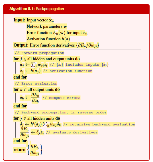
14.2 Backpropagation
Consider a feed-forward network. Each unit j receives a weighted sum of inputs a_j = \sum_i w_{ji} z_i where z_i is the output of another neuron (or an input unit) and w_{ji} is the weight of the connection from unit i to unit j. The output of unit j is obtained by applying the activation function h(\cdot): z_j = h(a_j)
Training the network proceeds in three steps, repeated for each data point n in the training set.
14.2.1 Step 1 — Forward propagation
We supply the input vector to the network and compute the activations of all neurons (hidden and output), layer by layer, to obtain the prediction z_k for each output unit k.
14.2.2 Step 2 — Computing \delta for the output units
Now that we have the prediction, we want to compute how the error E_n changes with respect to each weight w_{ji}. By the chain rule, we can decompose this derivative into two factors: \dfrac{\partial E_n}{\partial w_{ji}} = \underbrace{\dfrac{\partial E_n}{\partial a_{j}}}_{\delta_j} \cdot \underbrace{\dfrac{\partial a_j}{\partial w_{ji}}}_{z_i} The first factor measures how sensitive the error is to the total input a_j of unit j; we call it \delta_j. The second factor is simply z_i, the output of the unit sending the signal (since a_j = \sum_i w_{ji} z_i, differentiating with respect to w_{ji} leaves only z_i).
Therefore, the gradient rule for any weight is: \dfrac{\partial E_n}{\partial w_{ji}} = \delta_j \cdot z_i
For the output units, \delta is computed directly from the loss. For example, with MSE: \delta_{k} = \dfrac{\partial E_n}{\partial a_{k}} = (z_k - t_k) \cdot h'(a_k) \quad \forall k \in \text{output units}
14.2.4 Weight update
Once all \delta’s have been computed, the gradient of every weight is already known: \dfrac{\partial E_n}{\partial w_{ji}} = \delta_j \cdot z_i
and the weights are updated via gradient descent: w_{ji} \leftarrow w_{ji} - \mu \dfrac{\partial E_n}{\partial w_{ji}}
Example The network has the following architecture:
- Input Layer: 2 input nodes, I_1, I_2.
- Hidden Layer 1: 2 neurons, K and M.
- Hidden Layer 2: 2 neurons, P and Q.
- Output Layer: 1 neuron, O.
Notation:
- W_{ij} is the weight of the connection from node i to node j.
- a_j is the weighted sum of inputs to neuron j.
- h(x) is the activation function (e.g., sigmoid).
- h'(x) is its derivative.
- z_j = h(a_j) is the output of neuron j.
- t is the target (desired) value for the single output.
- E is the error (or cost) function. We will use the Mean Squared Error (MSE): E = \frac{1}{2}(z_o - t)^2.
14.2.5 1. Forward Propagation
We calculate the output of each neuron, layer by layer, until we reach the final output.
Hidden Layer 1: a_k = W_{1k} I_1 + W_{2k} I_2, \quad z_k = h(a_k) a_m = W_{1m} I_1 + W_{2m} I_2, \quad z_m = h(a_m)
Hidden Layer 2: a_p = W_{kp} z_k + W_{mp} z_m, \quad z_p = h(a_p) a_q = W_{kq} z_k + W_{mq} z_m, \quad z_q = h(a_q)
Output Layer (1 neuron O): a_o = W_{po} z_p + W_{qo} z_q, \quad z_o = h(a_o)
14.2.6 2. Backward Propagation (Backpropagation)
The goal is to calculate the gradient of the error function with respect to each weight in the network (\frac{\partial E}{\partial W_{ij}}) in order to update them. We proceed backward, from the output layer to the input layer.
14.2.7 Defining the Error and Delta (\delta) Terms
The fundamental rule for updating a weight W_{ij} is derived from the chain rule: \frac{\partial E}{\partial W_{ij}} = \frac{\partial E}{\partial a_j} \frac{\partial a_j}{\partial W_{ij}}
We define the “delta” term as \delta_j = \frac{\partial E}{\partial a_j}. Since a_j = \sum_i W_{ij}z_i, its partial derivative with respect to the weight W_{ij} is simply the input activation z_i. The rule becomes:
\frac{\partial E}{\partial W_{ij}} = \delta_j \cdot z_i
14.2.8 Calculating the Delta Terms
We calculate the \delta terms starting from the last layer.
1. Delta of the Output Node (O)
\delta_o = \frac{\partial E}{\partial a_o} = \frac{\partial E}{\partial z_o} \frac{\partial z_o}{\partial a_o}
With E = \frac{1}{2}(z_o - t)^2, we have \frac{\partial E}{\partial z_o} = (z_o - t). The derivative of the activation is \frac{\partial z_o}{\partial a_o} = h^{'}(a_o). Thus:
\delta_o = (z_o - t) \cdot h^{'}(a_o)
2. Deltas of Hidden Layer 2 Nodes (P and Q)
The error at node P is determined by how it contributes to the error at node O.
\delta_p = \frac{\partial E}{\partial a_p} = \frac{\partial E}{\partial a_o} \frac{\partial a_o}{\partial z_p} \frac{\partial z_p}{\partial a_p} = (\delta_o \cdot W_{po}) \cdot h^{'}(a_p)
Rewriting in the standard form:
\delta_p = h'(a_p) \cdot (W_{po} \cdot \delta_o)
Similarly for node Q:
\delta_q = h^{'}(a_q) \cdot (W_{qo} \cdot \delta_o)
3. Deltas of Hidden Layer 1 Nodes (K and M)
The error at node K is determined by how it contributes to the errors at both P and Q.
Substituting the terms:
\delta_k = \frac{\partial E}{\partial a_k} = \left( \frac{\partial E}{\partial a_p}\frac{\partial a_p}{\partial z_k} + \frac{\partial E}{\partial a_q}\frac{\partial a_q}{\partial z_k} \right) \cdot \frac{\partial z_k}{\partial a_k}
\delta_k = (\delta_p \cdot W_{kp} + \delta_q \cdot W_{kq}) \cdot h'(a_k)
Rewriting in the standard form:
\delta_k = h'(a_k) \cdot (W_{kp} \cdot \delta_p + W_{kq} \cdot \delta_q)
14.2.9 Full Gradient Derivation for a Weight (Example: \frac{\partial E}{\partial W_{1k}})
As shown in your notes, let’s derive the full expression for the gradient with respect to the weight W_{1k}, which connects input I_1 to neuron K.
The basic rule is:
\frac{\partial E}{\partial W_{1k}} = \delta_k \cdot I_1
Now, we substitute the delta terms backward through the network.
Step 1: Substitute \delta_k
\frac{\partial E}{\partial W_{1k}} = \left[ h'(a_k) \cdot (W_{kp} \cdot \delta_p + W_{kq} \cdot \delta_q) \right] \cdot I_1
Step 2: Substitute \delta_p and \delta_q
\frac{\partial E}{\partial W_{1k}} = \left[ h'(a_k) \cdot (W_{kp} \cdot [h'(a_p) \cdot W_{po} \cdot \delta_o] + W_{kq} \cdot [h'(a_q) \cdot W_{qo} \cdot \delta_o]) \right] \cdot I_1
Step 3: Factor out the common term \delta_o
\frac{\partial E}{\partial W_{1k}} = \left[ h'(a_k) \cdot \left( W_{kp} h'(a_p) W_{po} + W_{kq} h'(a_q) W_{qo} \right) \cdot \delta_o \right] \cdot I_1
Step 4: Substitute the final expression for \delta_o
\frac{\partial E}{\partial W_{1k}} = \left[ h'(a_k) \cdot \left( W_{kp} h'(a_p) W_{po} + W_{kq} h'(a_q) W_{qo} \right) \cdot \left( (z_o - t) \cdot h'(a_o) \right) \right] \cdot I_1
Final, Reordered Expression:
This complete expression shows how an error at the output (z_o - t) is propagated backward through all paths to determine the impact of a single weight in the first layer. \frac{\partial E}{\partial W_{1k}} = I_1 \cdot h'(a_k) \cdot \left( W_{kp} h'(a_p) W_{po} + W_{kq} h'(a_q) W_{qo} \right) \cdot (z_o - t) h'(a_o)