12 Probabilistic Graphical Models
Probability theory can be expressed in terms of two simple equations:
\text{sum rule} \quad p(X) = \sum_Y p(X, Y) \text{product rule} \quad p(X, Y) = p(Y | X) p(X)
All of the probabilistic manipulations, no matter how complex, amount to repeated application of these two equations. We use diagrammatic representations of probability distributions as these offer the following properties:
- They provide a simple way to visualize the structure of a probabilistic model
- Insights into the properties of the model can be obtained by inspecting the graph
- The computations required to perform inference and learning can be expressed in terms of graphical operations
In a probabilistic graphical model, each node represents a random variable, and the links express probabilistic relationships between these variables. The graph then captures the way in which the joint distribution over all the random variables can be decomposed into a product of factors each depending only on a subset of the variables.
12.1 Bayesian Networks
A Bayesian Network is a directed acyclic graph. To motivate the use of directed graphs to describe probability distributions, consider first an arbitrary joint distribution p(a, b, c) over three variables a, b, and c. By application of the product rule: p(a, b, c) = p(c | a, b) p(b) p(a) = p(c | a, b) p(b | a) p(a)
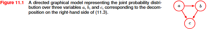
Now we represent the right-hand side as follows: we introduce a node for each random variable, and associate each node with the corresponding conditional distribution on the right-hand side. For each conditional distribution, we add directed links from the nodes corresponding to the variables on which the distribution is conditioned. For the factor p(c | a, b) there will be links from nodes a and b to node c, whereas for the factor p(a) there will be no incoming links.
Formally, the joint distribution defined by a graph is given by the product, over all of the nodes of the graph, of a conditional distribution for each node conditioned on the variables corresponding to the parents of that node in the graph.
p(x_1, ..., x_K) = \prod_{k = 1}^K p(x_k | pa(k))
pa(k) denotes the set of parents of x_k. This equation expresses the factorization properties of the joint distribution for a directed graphical model.
12.1.1 Discrete Variables
The probability distribution p(x | \mu) for a single discrete variable x having K possible states is given by p(x | \mu) = \prod_{k = 1}^K \mu_k^{x_k}
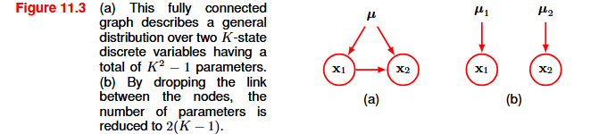
and is governed by the parameters \mu = (\mu_1, ..., \mu_K) ^T. Due to the constraint \sum_k \mu_k = 1, only K - 1 values for \mu_k need to be specified. If we want to model the joint distribution between two discrete variables, x_1 and x_2, each of which has K states, we will have
p(x_1, x_2 | \mu) = \prod_{k = 1}^K \prod_{l = 1}^K \mu_{kl}^{x_{1k} x_{2l}}
This distribution is governed by K^2 - 1 parameters. So an arbitrary joint distribution over M variables has K^M - 1 parameters, and therefore grows exponentially with the number M of variables.
If we consider M independent variables, we will have M(K - 1) parameters, which therefore grow linearly with the number of variables. We reduce the number of parameters by dropping links in the graph, at the expense of having a more restricted class of distributions.
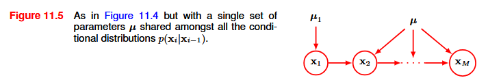
An alternative way to reduce the number of parameters is by sharing parameters, so that some conditional distributions are governed by the same set of parameters.
12.2 Conditional Independence
Consider three variables a, b, and c, and suppose that the conditional distribution of a given b and c is such that it does not depend on the value of b, so that p(a | b, c) = p(a | c) We say that a is conditionally independent of b given c.
12.2.1 D-Separation
Two nodes, X and Y, are d-separated by a set of evidence nodes Z if and only if every path between X and Y is blocked.
A path is blocked if at least one of these conditions is true:
- The path contains a chain (A → B → C) where the middle node B is in the conditioning set Z.
- The path contains a fork (A ← B → C) where the middle node B is in the conditioning set Z.
- The path contains a collider (A → B ← C) where the collider B is NOT in the conditioning set Z, and none of B’s descendants are in Z either.
D-Separation is used to check whether two nodes are conditionally independent in a graphical model, given a set of observed variables. If two nodes are d-separated by the observed variables, then they are conditionally independent given those variables.
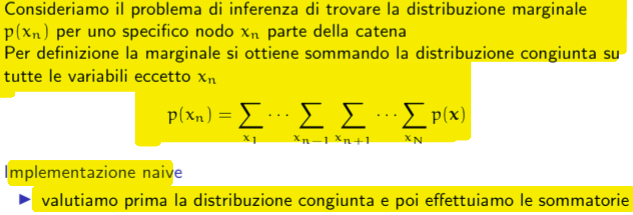
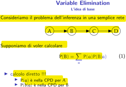
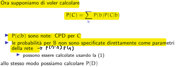
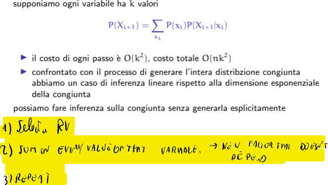
12.3 Inference
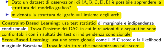
12.4 Structure learning
12.5 Naive Bayes
In a naive Bayes model, we use conditional independence assumptions to simplify the model structure. We define a class-conditional density p(x | C_k) for each class, along with prior class probabilities p(C_k). The key assumption is that, conditioned on the class C_k, the distribution of the input variable factorizes into a product of component densities. Suppose we partition x into L elements \mathbf{x} = (x^{(1)}, ..., x^{(L)}); for each class, Naive Bayes takes the form
p(x | C_k) = \prod_{l = 1}^L p(x^{(l)}| C_k)
We can fit the naive Bayes model to the training data using maximum likelihood by assuming that the data are drawn independently from the model. This is done by fitting the model for each class separately using the corresponding labelled data, and then setting the class priors p(C_k) equal to the number of training data points in each class. The probability that x belongs to class C_k is then given by Bayes’ theorem:
p(C_k | x) = \dfrac{p(x | C_k) p(C_k)}{p(x)} = \dfrac{p(x | C_k) p(C_k)}{\sum_{k = 1}^K p(x | C_k) p(C_k)}
The naive Bayes assumption is helpful when the dimensionality D of the input space is high, making density estimation in the full D-dimensional space more challenging. It is also useful if the input vector contains both discrete and continuous variables, since each can be represented separately using appropriate models. Even with the strong assumption of conditional independence, the model may still give good classification performance in practice.