7  Support Vector Machines

7.1 Lagrange Multipliers

Lagrange multipliers are a technique to find the stationary points of a function subject to constraints. They are the mathematical backbone behind SVMs.

7.1.1 Equality Constraints

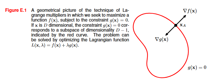
Consider the problem \max f(x_1, x_2) \quad \text{subject to} \; g(x_1, x_2) = 0 At a constrained optimum, the gradients \nabla f(x) and \nabla g(x) must be parallel (otherwise we could move along the constraint surface and still improve f). So there exists a scalar \lambda, called Lagrange multiplier, such that \nabla f + \lambda \nabla g = 0. We capture this by defining the Lagrangian \mathcal{L}(x, \lambda) = f(x) + \lambda g(x) and solving \nabla \mathcal{L} = 0 with respect to both x and \lambda.

7.1.2 Inequality Constraints

Now consider maximizing f(x) subject to g(x) \geq 0. Two cases arise:

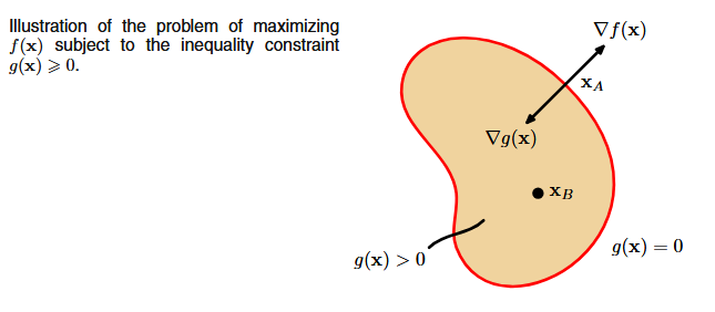
• Inactive constraint (g(x^*) > 0): the optimum lies inside the feasible region, so the constraint doesn’t matter. We simply solve \nabla f = 0, and \lambda = 0.
• Active constraint (g(x^*) = 0): the optimum sits on the boundary. Here \nabla f must point out of the feasible region (we can’t improve further), which means \nabla f and \nabla g are anti-parallel, so \lambda > 0.

Both cases are unified by the Karush-Kuhn-Tucker (KKT) conditions. We optimize \mathcal{L}(x, \lambda) = f(x) + \lambda g(x) subject to:

1. g(x) \ge 0, i.e. the original constraint holds
2. \lambda \ge 0, which combines \lambda = 0 (inactive) and \lambda > 0 (active)
3. \lambda \, g(x) = 0, known as complementary slackness: at least one of \lambda or g(x) must be zero

These conditions (plus \nabla_x \mathcal{L} = 0) let us find the solution without guessing whether the constraint is active or not.

Note: For minimization with g(x) \ge 0, we minimize \mathcal{L}(x, \lambda) = f(x) - \lambda g(x) instead. For multiple constraints g_j(x) = 0 and h_k(x) \ge 0, we introduce one multiplier per constraint: \mathcal{L} = f(x) + \sum_j \lambda_j g_j(x) + \sum_k \mu_k h_k(x) with KKT conditions \mu_k \ge 0 and \mu_k h_k(x) = 0 for each inequality constraint.

7.2 Support Vector Machines

7.2.1 Hard Margin SVM

Consider a two-class classification problem with a linear model y(x) = w^T \phi(x) + b, where \phi(x) maps inputs to a feature space. We classify new points by \text{sign}(y(x)), with targets t_n \in \{-1, +1\}.

If the data is linearly separable, there are infinitely many hyperplanes that separate the classes. Which one should we pick? The one that gives the largest margin, meaning the largest gap between the decision boundary and the nearest data points. Intuitively, a wider margin means more confidence and better generalization.

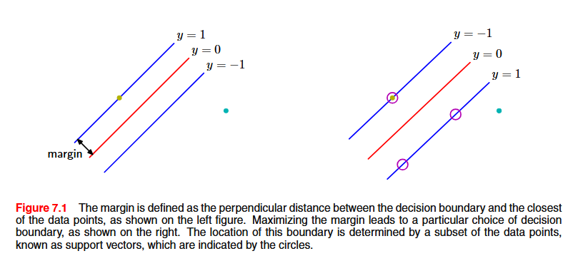
The perpendicular distance of a correctly classified point x_n to the decision boundary is \frac{t_n(w^T\phi(x_n) + b)}{||w||} We want to maximize the distance to the closest point. By rescaling w and b, we can always set t_n(w^T\phi(x_n) + b) = 1 for the closest points. Then all points satisfy t_n(w^T\phi(x_n) + b) \ge 1, and the margin becomes \frac{2}{||w||}. Maximizing this is equivalent to:

\min_{w,b} \; \frac{1}{2} ||w||^2 \quad \text{subject to} \quad t_n(w^T\phi(x_n) + b) \ge 1, \;\; \forall \, n

This is the hard margin SVM: no training errors are allowed. We can express this as minimizing \sum_{n=1}^N E_{\infty}(t_n y(x_n) - 1) + \frac{1}{2} ||w||^2 where E_{\infty} is a loss that returns 0 when its argument is non-negative (the point satisfies the margin) and \infty when it is negative (the point violates the margin). In other words, any single violation makes the total cost infinite, so the optimizer is forced to classify every point correctly.

7.2.2 The Dual Problem

Introducing Lagrange multipliers a_n \ge 0 (one per constraint) and applying the KKT conditions, we can reformulate the problem into its dual form:

\max_a \; \sum_{n=1}^{N} a_n - \frac{1}{2} \sum_{n,m} a_n a_m t_n t_m k(x_n, x_m) \quad \text{s.t.} \quad a_n \ge 0, \;\; \sum_n a_n t_n = 0

where k(x_n, x_m) = \phi(x_n)^T \phi(x_m) is the kernel function. This is a quadratic programming problem.

Why bother with the dual? Two key reasons:

• The data appears only through inner products k(x_n, x_m), enabling the kernel trick
• The solution is sparse: most a_n = 0, meaning most data points don’t affect the model

The KKT conditions tell us: a_n \ge 0, \quad t_n y(x_n) - 1 \ge 0, \quad a_n(t_n y(x_n) - 1) = 0 So either a_n = 0 (the point doesn’t contribute) or t_n y(x_n) = 1 (the point lies exactly on the margin). The points with a_n > 0 are the support vectors, and only these matter for predictions.

7.2.3 Kernel Trick

The dual formulation depends on the data only through inner products \phi(x_n)^T\phi(x_m), which can be replaced by a kernel function k(x_n, x_m). This allows SVMs to operate in high-dimensional (even infinite-dimensional) feature spaces without ever computing \phi(x) explicitly.

In practice, this means we can create non-linear decision boundaries by choosing an appropriate kernel (e.g., polynomial, RBF), while the optimization problem stays the same.

7.2.4 Classification

New data points are classified using: y(x) = \sum_{n \in \text{SV}} a_n \, t_n \, k(x, x_n) + b where the sum runs only over support vectors. The bias b is computed by averaging over all support vectors (which satisfy t_n y(x_n) = 1): b = \frac{1}{N_S}\sum_{n \in S}\left(t_n - \sum_{m \in S} a_m \, t_m \, k(x_n, x_m)\right)

7.2.5 Soft Margin: Handling Non-Separable Data

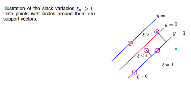
Real data is rarely perfectly separable. We relax the hard constraints by introducing slack variables \xi_n \ge 0:

t_n y(x_n) \ge 1 - \xi_n

• \xi_n = 0: correctly classified, on or beyond the margin
• 0 < \xi_n \le 1: inside the margin but on the correct side
• \xi_n > 1: misclassified

We now minimize: \min_{w,b,\xi} \; \frac{1}{2} ||w||^2 + C\sum_{n=1}^N \xi_n \quad \text{s.t.} \quad t_n y(x_n) \ge 1 - \xi_n, \;\; \xi_n \ge 0

The parameter C > 0 controls the trade-off: large C penalizes errors heavily (narrow margin, few violations); small C tolerates more errors (wider margin). Think of C as the inverse of a regularization coefficient.

Note that the slack variable \xi_n is exactly the hinge loss \max(0, \; 1 - t_n y(x_n)): it is zero when the point is correctly classified beyond the margin, and grows linearly as it violates. So the soft margin SVM is equivalent to minimizing \sum_{n=1}^N \max(0, \; 1 - t_n y(x_n)) + \frac{1}{2}||w||^2

The dual problem has the same form as before, with one change: a_n is now bounded above by C: \max_a \; \sum_{n=1}^{N} a_n - \frac{1}{2} \sum_{n,m} a_n a_m t_n t_m k(x_n, x_m) \quad \text{s.t.} \quad 0 \le a_n \le C, \;\; \sum_n a_n t_n = 0

Predictions use the same formula. The bias b is computed using points with 0 < a_n < C.

7.3 Regression (SVR)

For regression, we replace the standard squared-error loss with an \epsilon-insensitive loss: predictions within \epsilon of the target incur zero loss.

E_\epsilon(y(x) - t) = \begin{cases} 0, & \text{if } |y(x) - t| < \epsilon \\ |y(x) - t| - \epsilon, & \text{otherwise} \end{cases}

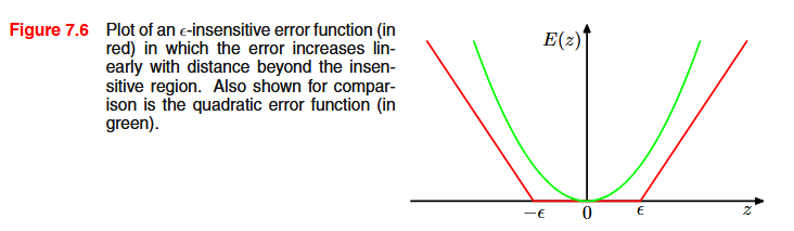
This creates a “tube” of width 2\epsilon around the regression line. Points inside the tube are considered “good enough” and don’t contribute to the loss.

Since violations can go in both directions, we need two sets of slack variables: \xi_n for points above the tube and \hat{\xi}_n for points below.

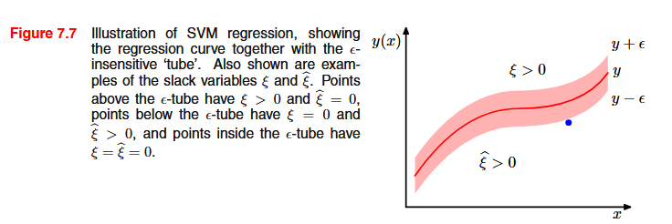
The optimization problem becomes: \min_{w,b,\xi,\hat{\xi}} \; \frac{1}{2} ||w||^2 + C\sum_{n=1}^N (\xi_n + \hat{\xi}_n) \quad \text{s.t.} \quad \begin{cases} t_n \le y(x_n) + \epsilon + \xi_n \\ t_n \ge y(x_n) - \epsilon - \hat{\xi}_n \\ \xi_n, \hat{\xi}_n \ge 0 \end{cases}

The dual introduces two multipliers per point (a_n and \hat{a}_n): \max_{a, \hat{a}} \; -\frac{1}{2} \sum_{n,m} (a_n - \hat{a}_n)(a_m - \hat{a}_m) k(x_n, x_m) - \epsilon \sum_n (a_n + \hat{a}_n) + \sum_n (a_n - \hat{a}_n) t_n \text{s.t.} \quad 0 \le a_n, \hat{a}_n \le C, \quad \sum_n (a_n - \hat{a}_n) = 0

Predictions use: y(x) = \sum_{n \in \text{SV}} (a_n - \hat{a}_n) \, k(x, x_n) + b

Support vectors are the points lying on or outside the \epsilon-tube (those with a_n > 0 or \hat{a}_n > 0). Again, the solution is sparse.

7.4 Summary

Definition. SVMs are supervised models that find the optimal hyperplane y(x) = w^T\phi(x) + b by maximizing the margin between classes (classification) or fitting an \epsilon-insensitive tube (regression).

Support Vectors. The data points with non-zero Lagrange multipliers (a_n \neq 0). Only these contribute to predictions; all other training points can be discarded. In classification they lie on the margin boundaries; in regression they lie on or outside the \epsilon-tube.

Kernel Trick. The dual formulation depends on data only through inner products \phi(x_n)^T\phi(x_m), replaceable by a kernel k(x_n, x_m). This lets SVMs work in high-dimensional feature spaces without computing \phi(x) explicitly, enabling non-linear boundaries at no extra cost.

Inference.

• Classification: \;\text{sign}\!\left(\displaystyle\sum_{n \in \text{SV}} a_n \, t_n \, k(x, x_n) + b\right)
• Regression: \;\displaystyle\sum_{n \in \text{SV}} (a_n - \hat{a}_n) \, k(x, x_n) + b

What we optimize.

Variant	Primal (minimize)	Dual (maximize)	Constraint on a_n
Hard margin	\frac{1}{2}\|w\|^2 s.t. t_n y(x_n) \ge 1	\sum a_n - \frac{1}{2}\sum_{n,m} a_n a_m t_n t_m k(x_n,x_m)	a_n \ge 0
Soft margin	\frac{1}{2}\|w\|^2 + C\sum \xi_n s.t. t_n y(x_n) \ge 1 - \xi_n	same form	0 \le a_n \le C
SVR	\frac{1}{2}\|w\|^2 + C\sum(\xi_n + \hat\xi_n)	see regression dual	0 \le a_n, \hat{a}_n \le C

7.5 Appendix: Derivazione del Duale

Il problema primale è: \min_{w,b} \; \frac{1}{2} ||w||^2 \quad \text{subject to} \quad t_n(w^T\phi(x_n) + b) \ge 1, \;\; \forall \, n

Non possiamo risolverlo con una semplice derivata perché ci sono vincoli di disuguaglianza. Introduciamo un moltiplicatore di Lagrange a_n \ge 0 per ogni vincolo, ottenendo il Lagrangiano: L(w, b, a) = \frac{1}{2}||w||^2 - \sum_{n=1}^N a_n \left[t_n(w^T\phi(x_n) + b) - 1\right]

Espandiamolo: L = \frac{1}{2}w^Tw - \sum_n a_n t_n w^T\phi(x_n) - b\sum_n a_n t_n + \sum_n a_n

Derivata rispetto a w: \frac{\partial L}{\partial w} = w - \sum_n a_n t_n \phi(x_n) = 0 \quad \Rightarrow \quad w = \sum_n a_n t_n \phi(x_n)

Derivata rispetto a b: \frac{\partial L}{\partial b} = -\sum_n a_n t_n = 0 \quad \Rightarrow \quad \sum_n a_n t_n = 0

Sostituzione. Ora rimpiazziamo w e usiamo \sum_n a_n t_n = 0 dentro L. Nella sostituzione usiamo l’indice m per la seconda somma, per distinguerla dalla somma su n già presente (sono due indici indipendenti che scorrono entrambi da 1 a N).

Termine 1: b\sum_n a_n t_n sparisce perché \sum_n a_n t_n = 0.

Termine 2: \frac{1}{2}w^Tw. Sostituiamo w = \sum_n a_n t_n \phi(x_n): \frac{1}{2}w^Tw = \frac{1}{2}\left(\sum_n a_n t_n \phi(x_n)\right)^T\left(\sum_m a_m t_m \phi(x_m)\right) Distribuiamo il prodotto (ogni elemento della prima somma moltiplica ogni elemento della seconda): = \frac{1}{2}\sum_n \sum_m a_n a_m t_n t_m \, \phi(x_n)^T\phi(x_m) = \frac{1}{2}\sum_{n,m} a_n a_m t_n t_m \, k(x_n, x_m)

Termine 3: \sum_n a_n t_n w^T\phi(x_n). Anche qui sostituiamo w: \sum_n a_n t_n w^T\phi(x_n) = \sum_n a_n t_n \left(\sum_m a_m t_m \phi(x_m)\right)^T \phi(x_n) Distribuiamo come prima: = \sum_n \sum_m a_n a_m t_n t_m \, \phi(x_m)^T\phi(x_n) = \sum_{n,m} a_n a_m t_n t_m \, k(x_n, x_m)

Termine 4: \sum_n a_n resta invariato.

Ricombiniamo. L era \text{Termine 2} - \text{Termine 3} + \text{Termine 4}: L = \frac{1}{2}\sum_{n,m} a_n a_m t_n t_m \, k(x_n, x_m) - \sum_{n,m} a_n a_m t_n t_m \, k(x_n, x_m) + \sum_n a_n = -\frac{1}{2}\sum_{n,m} a_n a_m t_n t_m \, k(x_n, x_m) + \sum_n a_n = \sum_n a_n - \frac{1}{2}\sum_{n,m} a_n a_m t_n t_m \, k(x_n, x_m)

I dati compaiono solo come k(x_n, x_m) = \phi(x_n)^T\phi(x_m): è qui che si sblocca il kernel trick.