7 Data Streams
7.1 Tasks
- Cluster analysis
- Predictive analysis
- Monitoring evolution/Change detection
- Detect changes in the behavior of sensors
- Detect failures and abnormal activities
- Detect extreme values, anomalies and outliers detection
7.2 Data Streams Models
The standard approach is to select a finite sample of data, generate a static model and apply it. The problem is that the world is not static and things change over time.
A data stream is a continuous flow of data generated at high speed in dynamic, time-changing environments.
The usual approaches used for batch procedures cannot cope with this streaming setting. Machine Learning algorithms assume
- Instances are independent and generated at random according to some probability distribution D
- D is stationary
- The training set is finite
With data streams, decision models must be capable of
- Incorporating new information at the speed data arrives
- Detecting changes and adapting the model to the most recent information
- Forgetting outdated information
The training set is unbounded.
The input elements arrive sequentially by timestamp, and describe an underlying function A that can be:
- Insert Only model: once an element is seen it cannot be changed: the knowledge I extract from every element cannot be removed, but only approximated
- Insert-Delete model: elements can be deleted but not updated
- We do not have update model, because data are in continuous flow, so updating an element is equivalent to deleting the old one and inserting the new one.
To deal with streaming data we need a Data Streams Management Systems, where queries are continuous, access is sequential, and data characteristics and arrival patterns are unpredictable. Cassandra can handle data streams.
Given the massive data streams, we want to use one-pass algorithms that can process data in a single pass, using limited memory and time per item, and give as output an approximate answer (with some error bound).
We define a synopsis as a compact summary of the data that can be used to answer queries approximately. A synopsis in the data stream model is a compact summary structure that maintains the essential characteristics of a continuous, potentially unbounded data stream using limited memory.
The answer we will give are like: Actual answer is within 5 \pm 1 with probability \leq 0.9.
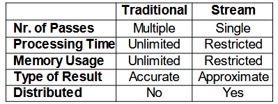
Algorithms that process data streams are typically sub-linear in time and space, but they provide an approximate answer. There are three constraints to consider: the amount of memory used to store information, the time to process each data element, and the time to answer the query of interest. In general, we can identify two parameters that define the quality of the approximation:
- Approximation \epsilon: the answer is correct within some small fraction \epsilon of error
- Answer is within 1 \pm \epsilon of the correct result
- Randomization \delta: allow a small probability of failure
- Answer is correct, except with probability 1 in \delta
- Success probability: (1 - \delta)
These two constant have influence on the space used for the synopsis. Typically, the space is O\left( \dfrac{1}{\epsilon^2} \log \left( \dfrac{1}{\delta} \right) \right).
7.3 Learning from Data Streams: Desirable Properties
When learning from data streams, algorithms should satisfy the following desirable properties:
- Processing each example in small constant time, fixed amount of main memory, single scan of the data without revisiting old records, processing examples at the speed they arrive
- Ability to detect and react to concept drift
- Decision models active anytime, they must not go offline for retraining
- Ideally, produce a model equivalent to the one that would be obtained by batch algorithms
7.4 Count-Min Sketch
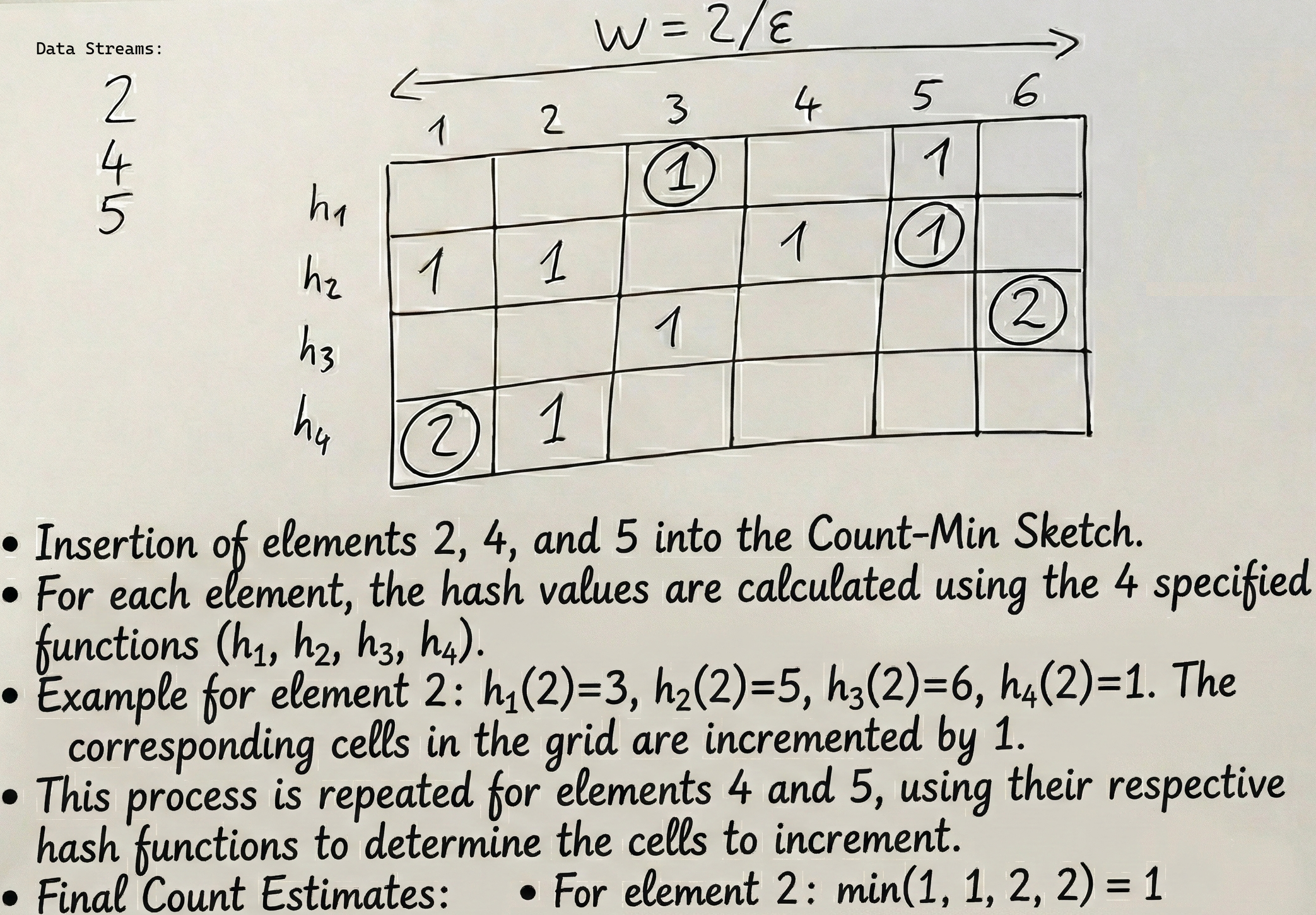
Count-Min Sketch is a probabilistic data structure that serves as a frequency table of events in a data stream. It uses hash functions to map events to counts in a two-dimensional array.
A Count-Min Sketch is an array of w \cdot d in size. Given a desired probability level (\delta), and an admissible error (\epsilon), the size of the data structure is w = \dfrac{2}{\epsilon} and d = \lceil \log\left(\dfrac{1}{\delta}\right) \rceil. Associated with each row there is a hash function h(.) that uniformly maps a value x to a value in the interval [1, ..., w].
Each entry x in the stream is mapped to one cell per row of the array of counts. It uses d hash functions to map entries to [1, ..., w]. When an update c of item j arrives, c is added to each of these cells. c can be any value: positive values for inserts, and negative values for deletes.
At any time we can answer point queries like:
How many times have we observed a particular IP?
To answer the query, we determine the set of d cells to which each of the d hash-functions map: CM [k, h_k(IP)]. The estimate is given by taking the minimum value among these cells: \hat{x}[IP ] = \min(\text{CM} [k, h_k(IP )]).
This estimate is always optimistic, that is x[j] \leq \hat{x}[j], where x[j] is the true value, because we do not subtract anything, and if there is a collision we always overestimate. The estimate is upper bounded by \hat{x}[j] \leq x[j] + \epsilon \cdot ||x||_1, with probability 1 - \delta, that is, the estimate is at most equal to the true value, plus “noise”, which is not higher than \epsilon times the total sum of all the seen elements.
The “hope” is to not have collision on the min value. This hope is determined by the choice of \epsilon and \delta.
7.5 Time Windows
Instead of computing statistics over all the stream we can use models to consider only the most recent data points. The rationale is that most recent data are more relevant than older data. We have several window models: Landmark, Sliding, Tilted Windows.
7.5.1 Landmark Windows
Landmark windows compute statistics from a fixed starting point (landmark) to the current time. All data from the landmark to now is considered. We effectively compute the statistics incrementally on the last data point seen.
The recursive version of the sample mean is well known:
\bar{x}_i = \frac{(i-1) \cdot \bar{x}_{i-1} + x_i}{i} \tag{7.1}
In fact, to incrementally compute the mean of a variable, we only need to maintain in memory the number of observations (i) and the sum of the values seen so far \sum x_i.
The incremental version of the standard deviation is:
s_n^2 = \frac{n-2}{n-1} s_{n-1}^2 + \frac{1}{n} (x_n - \hat{x}_{n-1})^2 \tag{7.2}
For the correlation coefficient, given two variables x and y, we need to maintain the sum of each stream (\sum x_i \text{ and } \sum y_i), the sum of the squared values (\sum x_i^2 \text{ and } \sum y_i^2), and the sum of the crossproduct (\sum(x_i \cdot y_i)):
corr(x,y) = \frac{\sum(x_i \cdot y_i) - \frac{\sum x_i \cdot \sum y_i}{n}}{\sqrt{\sum x_i^2 - \frac{\sum x_i^2}{n}} \sqrt{\sum y_i^2 - \frac{\sum y_i^2}{n}}} \tag{7.3}
7.5.2 Sliding Windows
We can use a simple moving average:
SMA_t = \frac{1}{w} \sum_{i=t-w+1}^{t} x_i \tag{7.4}
where w is the window size.
We can also use a weighted moving average:
WMA_t = \frac{\sum_{i=0}^{w-1} weight_i \cdot x_{t-i}}{\sum_{i=0}^{w-1} weight_i} \tag{7.5}
Computing these statistics in sliding windows requires to maintain all the observations inside the window (space: O(w)).
A better alternative is the exponential moving average:
EMA_t = \alpha \cdot x_t + (1 - \alpha) \cdot EMA_{t-1} \tag{7.6}
where \alpha represents the degree of weighting decrease, a constant smoothing factor between 0 and 1. A higher \alpha discounts older observations faster.
It has the flaw (or feature) of having an “infinite memory”: a very old anomalous data point will continue to minimally influence the average forever, whereas in the SMA, once it leaves the window, it disappears completely.
We can also apply the following algorithm:
- Use buckets of exponentially growing sizes (2^0, 2^1, … 2^h) to store the data
- Each bucket has a time-stamp associated with it
- It is used to decide when the bucket is out of the window
7.5.3 Tilted Windows
Tilted windows store data at different levels of granularity. The most recent data is stored at the highest granularity, while older data is stored at lower granularity: for example, we can store data every minute for the last hour, every hour for the last day, every day for the last month, and so on.
7.6 Sampling
To obtain an unbiased sampling of the data, we need to know the length of the stream, so we need to modify the approach here.
The idea is to sample at periodic time intervals, in this way we slow down data (if I don’t take all of them I don’t have to process them, I’m in fact reducing the stream rate). This obviously involves a loss of information.
7.6.1 Reservoir Sampling
- Creates uniform sample of fixed size k
- Insert first k elements into sample
- Then insert i-th element with probability p_i = \dfrac{k}{i}
- Delete an instance at random
It’s provable that every new element has the same probability of being in the sample, because the probability of being inserted is \dfrac{k}{i}, and the probability of not being deleted later is \dfrac{i}{i+1} \cdot \dfrac{i+1}{i+2} \cdot ... \cdot \dfrac{n-1}{n} = \dfrac{i}{n}, so the total probability is \dfrac{k}{n}.
The problems of this algorithm is that we have low probability of detecting changes or anomalies, it’s hard to parallelize, and on big streams the probability of being in the sample is very low.
7.7 Decision Trees for Data Streams
Why decision trees? Because every leaf represents a local pattern, so a restricted view of the data, so if something changes in the data it will be reflected in some leaves only.
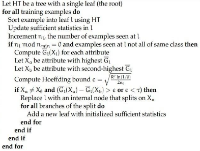
A successful example is the Very Fast Decision Tree system. The idea is that a small number of examples are enough to select the correct splitting test and expand a leaf. The algorithm split at a node only when there is enough statistical evidence in favor of that split.
Algorithm in brief:
- Collect sufficient statistics from a small set of examples (to recompute Gini/IG/Entropy)
- Estimate the merit of each attribute with Gini/IG/Entropy
- Use Hoeffding bound to statistically guarantee that the best attribute is better than the second best
- Let G(A_1) be the merit of the best attribute, and G(A_2) be the merit of the second best attribute
- Suppose we have n independent observations of a random variable r whose range is R. Let \bar{r} be the mean of these observations. Then, with probability 1 - \delta, the true mean of r is in the range \bar{r} \pm \epsilon, where \epsilon = \sqrt{\dfrac{R^2 \ln(1/\delta)}{2 n}} (Hoeffding bound)
- Hoeffding bound ensures that A_1 is the correct choice, with probability 1 - \delta, if (G(A_1) - G(A_2)) > \epsilon
Each leaf stores sufficient statistics to evaluate the splitting criterion. For continuous attributes we have a binary tree with counters of observed values, either single values or binned values. For nominal attributes we have the counter for each observed value per class.
VFDT assumes data is a sample drawn from a stationary distribution, but most data streams violate this assumption. We need to modify a bit the algorithm to deal with concept drift.
7.8 Concept Drift
Concept drift is the change of the underlying distribution that generates the data over time. Occurrences of drift can have impact in part of the instance space, whether globally (need to retrain) or locally (need to reconstruct parts).
7.8.1 Detecting Drift in VFDT
In the VFDT, each node can be equipped with a change detection algorithm to change the tree according to the new data distribution. So each node has a classifier that monitors if there is concept drift or not. If it is detected, the subtree rooted at that node is deleted and replaced with a new leaf computed with the new sufficient statistics.