1 NoSQL
1.1 Introduction
NoSQL Data Model diverges from the relational data model. Each NoSQL database has a different model:
- Key-Value
- Document
- Column-family
- Graph
- Sparse (index based)
The first three share a common characteristic, that is, the Aggregate Orientation
1.1.1 Relational vs Aggregate Model
The relational model takes the information that we want to store and divides it into tuples, that is a limited data structure because it captures a set of values, so, we can’t nest one tuple within another to get nested records, nor we can put a list of values or tuples within another. It allows us to think on data manipulation as operations that have as input tuples, and return tuples.
Aggregate orientation takes a different approach. It allows us to operate on data units having a more complex structure (list, map, nested data structures). Key-Value, document, and column-family databases use this complex structure. Given that we are talking about data unit, we would like to update aggregates with atomic operations (ACID properties respected on the whole complex object), we also want to communicate with our data storage in terms of aggregates. This kind of structure solves the impedance mismatch problem of relational databases, too.
1.1.2 Problem of classic relational models
- Relational mapping can capture any kind of relationships between entities but semantically we are not able to distinguish them, while if we work with aggregate-oriented databases, we have a clear view of the semantics of the data
- Relational databases are aggregate-ignorant, since they don’t have the concept of aggregate, same for graph databases. In domains where it is difficult to draw aggregate boundaries, aggregate-ignorant databases are useful.
- In general, aggregates may help in some operations and not in others (we can think of operations on data warehouses like sales in certain periods vs classic queries in relational databases that require joins)
- When there is no clear view, aggregate-ignorant databases are the best option
- But, remember the point that drove us to aggregate models, that is, scalability: running databases on a cluster is needed when dealing with huge quantities of data, it gives several advantages in computational power and data distribution, but we need to minimize the number of nodes to query when gathering data; if we explicitly include aggregates, we reinforce the ACID properties on the whole aggregate.
- Impedance w.r.t. the programming language: we need to map complex objects in the programming language to relations in the database, this requires extra code and effort.
- Relational models are oriented to help who designs the database to think in terms of relations, not who uses the database. In fact redundancies are avoided, data are normalized and complex queries are needed to retrieve data.
Note: Object relational model solves this problem by introducing the concept of complex object, but it still remains oriented to help who designs the database to think in terms of relations, not aggregates.
1.1.3 ACID Properties
- Atomic, consistent, isolated and durable
NoSQL aggregate databases can fail in a distributed environment because of consistency since they don’t support atomicity that spans multiple aggregates, because every transaction is made by a single object. So, if we need to update multiple aggregates we have to manage that in the application code and not at the database level. Thus atomicity is one of the considerations for deciding how to divide up our data into aggregates.
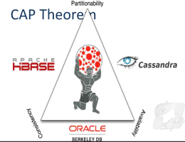
CAP Theorem: a distributed system can support only two of the following characteristics:
- Consistency: all copies have the same value. Not every question is answered (in small amount of time), but when answered, the answer is always correct
- Availability: system is fault-tolerant. Every question is answered but sometimes it has a wrong or outdated answer
- Partition tolerance: distribution of data, each system doesn’t influence the other
Very large systems will partition at some point, so partition tolerance must always be respected by NoSQL DBMS, so we need to choose between consistency and availability:
- Traditional DBMS (like relational ones) prefer consistency over availability
- Most web apps choose availability (e.g., e-commerce), unless for specific use cases.
1.2 Key-Value and Document-based databases
They differ in that:
- In a key-value the aggregate is opaque (BLOB)
- DBMS can’t understand what is inside the object, so we can’t query inside the object
- In a document database we can see the structure (JSON/XML)
- DBMS understands what is inside the object, so we can query inside the object.
- We need to enforce a structure in order to have a language to do queries
- DBMS understands what is inside the object, so we can query inside the object.
With a key-value we can only access by its key. With document we can submit queries based on fields, retrieve part of the aggregate, and create indexes based on the field of the aggregate.
1.2.1 Key-Value Databases
A KV store is a simple hash table where all the accesses to the database are via primary keys. A client can either:
- Get the value for a key in O(1)
- Put a value for a key in O(1)
- Delete a key in O(1)
The price to pay is redundancy: everything is stored as it will be queried. We design the structure based on the queries. Keys can be complex objects.
Key-value data access enables high performance and availability. Consistency is applicable only for operations on a single key.
The cons are:
- No complex query filters, all pass from the key to retrieve BLOBs
- All joins must be done at application level
- No foreign key constraints
- No triggers
The pros are:
- Efficient queries
- Easy to distribute
- Using a relational DB + cache forces into a KV storage anyway: we retrieve the data from the cache by key, if available, otherwise we run the query on the relational DB and cache the result. The difference is not here, but in how we interact and distribute the DB.
- No impedence mismatch.
DynamoDB is an example of a KV database. Dynamo treats both the key and the object supplied by the caller as an opaque array of bytes. It applies a MD5 hash on the key to generate a 128-bit identifier, which is used to determine the storage nodes that are responsible for serving the key. Dynamo relies on consistent hashing to distribute the load across multiple storage hosts. The output range of a hash function is treated as a fixed circular space called a ring.
Each node in the system is assigned a random value within this space which represents its position on the ring. Each data item is assigned to a node by:
- hashing the data item’s key to yield its position on the ring
- and then walking the ring clockwise to find the first node with a position larger than the item’s position.
Each node becomes responsible for the region in the ring between it and its predecessor node. The main advantage of consistent hashing is that departure or arrival of a node only affects its immediate neighbors.
1.2.2 Column-Family Stores
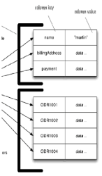
The name derives from the structure, composed of sparse columns and no schema. We don’t have to think of this structure as a table, but as a two-level map (map of maps). Columns put together form a family.
When is it better to store data as groups of columns rather than rows? When writing operations are rare but we need to read a few columns of many rows at once.
Column-family databases have a two-level aggregate structure. The first key is the row identifier, which returns a Map of columns. Once we fix a row, we can access all the column-families or a particular element.
This is the organization: the columns are organized into families, each column is a part of a family, and the column family acts as a unit of access. Then the data for a particular column family are accessed together.
We can model list based elements as a column-family. Thus we can have column-families with many elements and other with few elements. In Cassandra, we define:
- Skinny rows when we have few columns with the same columns used across the many different rows. In this case, the column family defines a record type, each row is a record, and each column is a field.
- Wide rows when we have many elements, with rows having very different columns. A wide column family models a list, with each column being one element in that list.
In skinny rows the column keys are ordered often by frequency, while in wide rows the column keys are ordered often by timestamp.
When we model data with column-family stores, we do it per query requirements. The general rule is to make it easy to query and denormalize data during writing.
NoSQL DBMSs are not suitable for systems:
- That require ACID transactions for writes and reads
- That need aggregation on the client side. A solution to this is to provide table with different aggregations (pre-aggregated data, problematic when data change frequently)
- That are in an initial stage. If we need to change the queries we could have to change the columns.
1.2.2.1 BigTable
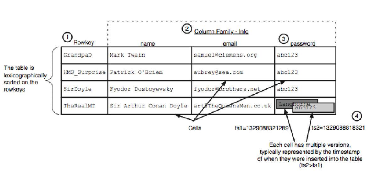
BigTable is a sparse, distributed, and persistent multi-dimensional sorted map. The map is indexed at the first level by a row-key, and at the second and third levels by a column-key and a timestamp, respectively. Each value in the map is an array of bytes.
(row: string, column: string, time: int64) -> string
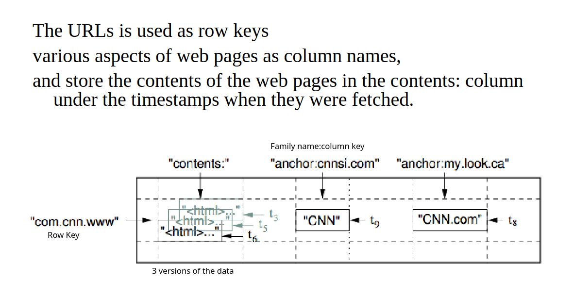
In the example, why do we use the reversed URL as the row key? Because in this way we can create row ranges called tablets, which are the units of distribution and load balancing. As a result, reads of short row ranges are efficient and typically require communication with a small number of machines. Reversing the URL we group into contiguous rows pages of the same domain.
The API supports:
- put(key, columnFamily, columnQualifier, value)
- get(key)
- Scan(startKey, endKey) (not O(1))
- delete(key)
BigTable uses a master-slave architecture based on the Google File System and a Distributed lock service, while Dynamo is P2P.
1.2.3 Graph Databases
We model all objects as nodes and relationships as edges. Relationships have types and directional significance. Relationships have names that let us traverse the graph. A query on the graph consists of traversing the graph from node to node via relationships, filtering nodes and relationships by their properties.
Relational DBs lack relationships (we cope with foreign keys and joins), NoSQL databases also lack relationships (there is no concept of relationship), while graph databases embrace relationships: nodes and edges are first-class citizens.
Graph databases try to preserve consistency and partitionability (Remember the CAP theorem):
- Consistency: since they operate on connected nodes, they could not scale well distributing nodes across servers
- Availability: Neo4j achieves availability by providing replicated slaves.
We can use relations to query graph-patterns in a very efficient way.
Indexes are necessary to find the starting node to be traversed. We can index properties of nodes and edges. Then, having a node, we can query both for incoming and outgoing relationships, so we can apply directional filters.
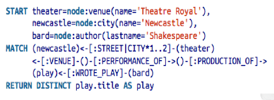
We use the MATCH to match patterns in relationships, the WHERE to filter the properties on a node or relationship, and the RETURN to specify what to get in the result set.
How do we model the world in graph terms?
Nodes contain properties. Think of nodes as documents that store properties in the form of arbitrary key-value pairs. The keys are strings and the values are arbitrary data types
Relationships connect and structure nodes, with a direction, a label, a start node and an end node, and properties. Properties are useful for
- Providing additional metadata
- Adding additional semantics (weights, costs, distances)
- Constraining queries at runtime