3 The KDD Process
We need a methodology that explains how data can be analyzed. This industrial methodology is known as Knowledge Discovery in Databases/Data (KDD).
Knowledge discovery is the nontrivial extraction of implicit, previously unknown, and potentially useful information from data.
- Nontrivial: some search or inference is involved, that is, it is not a straightforward computation (like computing an average).
- Implicit: information is not explicitly formulated in the data.
- Unknown: information should be novel and not present in the background knowledge.
- Useful: information extracted must be actionable (i.e., we create a model in order to deploy it).
Formally, given a set of facts (data) F, a representation language L to represent knowledge, and some measure of certainty C, we want to define a pattern as a statement S in L that describes relationships among a subset F_S of F, with a certainty c, such that S is simpler (in some sense) than the enumeration of all facts in F_S.
A pattern is considered knowledge if it is interesting and certain enough. Patterns are expressed in a high-level language L (e.g., rules, decision trees, etc.). Without sufficient certainty, they become unjustified. Certainty involves integrity of data, size of the sample on which the discovery was performed (less data -> ‘cleaner’ pattern, more data -> we can tolerate a wider margin of error), and the degree of support from available domain knowledge (how much is coherent with our background knowledge).
Patterns vs Models: a model is a global summary of the dataset, while a pattern is a local feature of the dataset (a subset of observations). In a decision tree, a single path of the tree is a pattern, the entire tree is the model. In a rule system, a single rule is a pattern, the whole set of rules is a model.
3.1 An Overview of the Process
KDD is an interactive and iterative process
- Developing an understanding of the application domain, the relevant background knowledge, and the goals of the end-user
- Creating a target data set: selecting a dataset, or focusing on a subset of variables or data samples
- Data cleaning and preprocessing: to remove noise or inconsistent data, and to transform the data into a suitable format for mining
- Data reduction and projection: finding useful features to represent the data depending on the goal of the task. Using multidimensionality reduction or transformation methods to reduce the effective number of variables under consideration
- Choosing the data mining task: deciding whether the goal of the KDD process is classification, regression, etc.
- Choosing the data mining algorithm(s): selecting the appropriate data mining algorithm(s) to be used for searching for patterns in the data
- Data mining: searching for patterns of interests in a particular representational form
- Interpreting mined patterns, possibly returning to any of steps 1–7 for further iteration
- Consolidating discovered knowledge: incorporating the knowledge in production.
This process has been consolidated by adding the business understanding as the first phase, and the deployment as the last phase, leading to the CRISP-DM methodology.
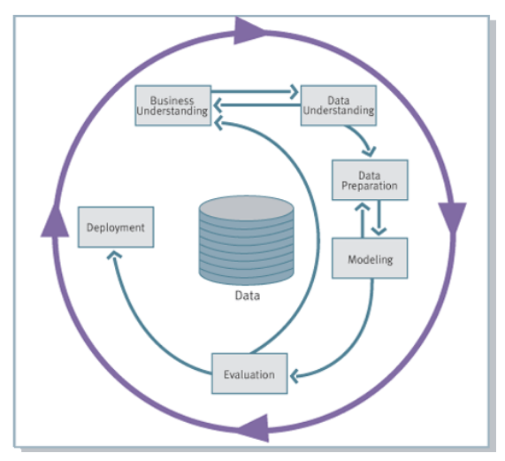
- The sequence is not strict, it is possible to move back and forth depending on the outcome of each phase. The arrows indicate the most important/frequent dependencies.
- The outer circle symbolizes the cyclic nature of a KDD process which can continue after a solution has been deployed.
- Each phase contains a number of tasks which produce specific outputs. In general, one report for every sub-phase.
Now let’s list the phases with the related sub-phases.
- Business Understanding
- Determine business objectives
- Assess situation
- Determine data mining goals
- Produce project plan
- Data Understanding
- Collect initial data
- Describe data
- Verify data quality
- Explore data
- Data Preparation
- Select data
- Sampling
- Feature selection
- Clean data
- Construct data
- Integrate data
- Format data
- Select data
- Modeling
- Select modeling techniques
- Generate test design
- Build model
- Assess model
- Evaluation
- Evaluate results
- Review process
- Deployment
- Plan deployment
- Monitoring and maintenance
- Produce Final report
- Review project
3.2 CRISP-DM: Business Understanding
3.2.1 Determine Business Objectives
We start from the minimum requirements:
- A perceived business problem or opportunity
- Some level of executive sponsorship: how important is it for the committee to introduce the technology (is it just to receive funds, or is it really useful for the company?)
It requires the collaboration of the business analyst and the data analyst.
This step is also the time at which we set the KPIs (Key Performance Indicators) for the project. KPIs are quantifiable measures that will be used as expectations for the project’s success. In KPIs, we consider also requirements like “reach an accuracy of X%”, not only business goals.
Output:
- The background, which details information about the business situation at the beginning of the process
- The business objectives, which describe primary goals from business perspectives
- The business success criteria (KPIs), which define measures for sufficiently high-quality results from a business point of view.
3.2.2 Assess Situation
We need to consider resources, constraints, assumptions, and other factors that may influence the project success.
Output:
- Inventory of:
- resources: personnel, software, hardware, data
- constraints: time, legal issues, budget
- assumptions: data availability, personnel availability
- A glossary of terminology, which covers both business and data mining terminology
- A cost-benefit analysis (drafted with the domain expert)
3.2.3 Determine Data Mining Goals
Business objectives (stated in business terms) have to be transformed into data mining goals (stated in technical terms). We need to map the objectives to a data mining task.
Typical data mining goals include:
- Supervised Learning: classification, estimation, prediction, forecasting, nowcasting
- Unsupervised Learning: affinity grouping (association rules, dependency modeling), clustering, profiling
- Summarization (or profiling) involves methods for finding a compact description for a subset of data, like statistics (mean, std, etc.) of all variables.
- Dependency modeling consists of defining a model that describes significant dependencies between variables. Dependency models exist at two levels:
- The structural level of the model specifies (often graphically, like Bayesian networks) which variables are locally dependent on each other
- The quantitative level specifies the strengths of the dependencies
- Drift detection: identifying changes in the distribution of data over time
- Change and deviation detection, like anomaly detection
Output:
- Data mining goals
- Success criteria for the data mining goals
3.2.4 Produce Project Plan
We describe the plan for achieving the data mining goals, and thereby achieving the business objectives.
Output:
- Project plan, like in a Gantt chart, which specifies the set of steps for the rest of the project, along with duration, required resources, inputs and outputs, and dependencies.
3.3 CRISP-DM: Data Understanding
3.3.1 Collect Initial Data
We need to access relevant data in the inventory of resources, like loading data from a data warehouse. Metadata collected in a data warehouse can help, like the data location (ETL processes).
Output:
- Initial data collection report, which describes the data sources, the data that has been collected and any problems encountered.
3.3.2 Describe Data
We need to examine the data in order to get familiar with it. This is the first time at which the properties of the data are examined.
There are two major types of variables:
- Categorical: the possible values are finite and differ in kind. There are two subtypes:
- Nominal: no order among the values (e.g., colors, names, etc.)
- Ordinal: there is an order (a total order relation) among the values (e.g., ratings like bad, good, excellent)
- Quantitative: arithmetic operations are allowed. There are two subtypes:
- Discrete: integers (e.g., number of children)
- Continuous: real numbers (e.g., height, weight, temperature)
Output:
- Data description report, which describes the data in terms of format, potential values, quantity, identities of the fields, and any surface information discovered (like columns with all the same value or all null values).
3.3.3 Verify Data Quality
Data quality is inspected, addressing the following issues:
- Accuracy: conformity of stored value to the actual value
- Completeness: no missing values
- Consistency: uniform representation (check if the temperature is always expressed in the same unit, etc.)
- Up-to-dateness: stored data is not obsolete
Poor data quality and poor data integrity are major issues in almost all KDD projects.
Output:
- Data quality report, which reports findings of the data quality verification. If quality problems exist, it also discusses possible solutions.
3.3.4 Explore Data
Data exploration starts here, combining statistical methods and data visualization techniques.
For categorical variables, frequency distributions of the values are a useful way of better understanding the data content. Histograms and pie charts help to identify distribution skews and invalid or missing values.
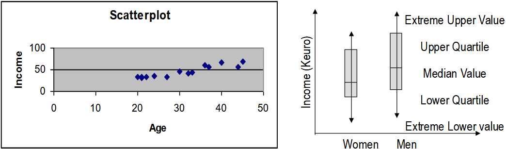
For quantitative variables, we are interested in max, min, mean, mode, median, std. When combined, these measures offer a powerful way of determining the presence of invalid and skewed data.
Other graphical tools are scatterplots, which represent the relationship between two or more continuous variables, and boxplots, useful for comparing the center (average) or spread (deviation) of two or more variables.
Output:
- Data exploration report.
3.4 CRISP-DM: Data Preparation
3.4.1 Select Data
Selection criteria include:
- Relevance to the data mining goals
- Quality and technical constraints (like if we have sensors, we need to consider their precision limits)
- Limits on data volumes or data types.
Data selection can be performed manually or automatically (sampling and feature selection).
3.4.1.1 Sampling
When the data volume is too high, we can extract a representative sample of the data.
The aim is to explain the variance of the data, no matter what techniques we adopt. So, if data are very noisy, we need more data to explain the variance. How large should the sample be? The tools to do this analysis fall under power analysis, and are based on estimates of means and variances of the variables in the population to be sampled. An alternative to setting a predetermined sample size is to let the data choose the size of the sample: the basic idea is to continue to increase the sample size until the results or summaries no longer change much. This is called progressive sampling.
3.4.1.1.1 Random Sampling
Every conceivable group of objects of the required size has the same chance of being selected. It is possible to get a very atypical sample; however, the laws of probability dictate that the larger a sample is, the more likely it will be representative of the population.
The main assumption of this technique (and the following ones in this paragraph) is that we are able to number the members of the target population in advance. So, this sampling is not always adequate, for example when dealing with data streams in which we don’t know the total size of data in advance, so we cannot ‘enumerate’ them.
This sampling can be done with or without replacement. If the population is large compared to the sample, there is a very small probability that any member will be chosen more than once, so the two methods are equivalent.
A variant of random sampling is stratified random sampling, which guarantees a fair representation of the population. The target population is divided into strata; then from each stratum we sample separately, and the union of all samples is the final sample.
We can control the number of observations within each stratum to ensure that particular groups are adequately represented in the sample. But every stratum has its own variance, so we may need a different number of samples from each stratum. Alternatively, we can sample the same number of observations from each stratum, but in this way we are corrupting the original distribution. The sample is usually proportional to the relative size of the strata; however, this is not a strict rule. Strata should be chosen to minimize variance within strata and maximize variance between strata (clustering, this is also called cluster sampling). Sample sizes should be proportional to the stratum standard deviation (more variance -> more samples).
In the context of large databases, a common application of cluster sampling is to randomly select blocks of data and then use all data in these blocks (block sampling). This kind of sampling can lead to biased samples if members of a cluster are more alike than members of different clusters.
3.4.1.1.2 Systematic Sampling
From now on, we don’t know the size of the population in advance.
Systematic sampling involves choosing one member at random from those numbered between 1 and k, then including every k-th member after this in the sample. For example, selecting every 10th record from a data stream.
This is easy to implement, even in data streams, but can lead to biased samples if there is an underlying pattern in the data that coincides with the sampling interval. It is especially vulnerable to periodicities. If periodicity is present and the period is a multiple of k, then we have bias; we are adding a new periodicity implicitly.
Another technique is two-stage sampling, in which we first select larger groups (clusters) of data, then we sample within these clusters. This is useful when we want to organize our sampling based on the values of one or more variables, but we do not know the range or distribution of these variables in the target population. An initial sample may facilitate more educated decisions about sampling strategies, so we use two-stage sampling as a preliminary step to choose which sampling strategy to use later.
3.4.1.1.3 Some Caveats
Many of the common tools for statistical inference, including t-tests, assume that the data comprise a simple random sample from some population, and that the individual data points are therefore statistically independent. Many of the sampling techniques will violate this assumption.
Random sampling provides unbiased estimates of the database, but if the database itself is a systematically biased sample from the real population, no statistical technique can rescue the resulting inferences.
3.4.1.2 Feature Selection
Feature selection is a process that chooses an optimal subset of features according to a certain criterion.
Problems of feature selection arise because
- Search complexity in the hypothesis space must be reduced for practical reasons
- Redundant or irrelevant features can have significant effects on the quality of the results of the analysis method. This problem is called curse of dimensionality.
Curse of dimensionality
The basic idea of the curse of dimensionality is that it is difficult to work on high-dimensional data for several reasons:
- The required number of samples grows exponentially with the number of variables
- There aren’t enough observations to get good estimates.
There are three main approaches to feature selection:
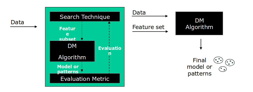
- Wrapper models: use a data mining algorithm to determine whether a subset of features is good. The same algorithm is used both for the feature selection and to obtain the final model, so it has to be as light as possible. The feature selection is performed as a search problem, where different combinations of features are prepared, evaluated, and compared to other combinations. They form a lattice structure, where each node is a subset of features. The search through the lattice can be performed with different strategies, like best-first search, A*, etc. The evaluation of a subset is performed by training and testing the model with only the features in the subset, and using the resulting accuracy as a measure of goodness. The search space is exponential.
- Filter models: are independent of the data mining algorithm that will use the subset of features. Subsets are evaluated using measures of intrinsic properties of the data, such as information measures or distance measures on probability distributions (KL divergence, etc.).
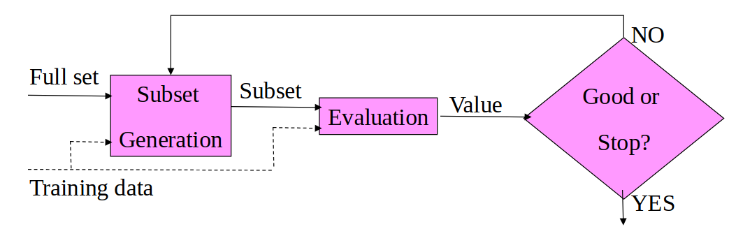
To generate the subsets we can enumerate them, take a random subset, or sequentially generate in forward selection or backward selection, whether we start from an empty set and add features, or start from the full set and remove features.
These strategies are based on a greedy search strategy in the space of 2^N subsets, where N is the number of features in the original dataset.
To evaluate the quality:
Information measures: Information Gain IG(X) = \sum_i U(P(c_i)) - E[\sum_i U(P(c_i|X))], where U is the uncertainty function, P(c_i) are the prior class probabilities of the features that we want to consider. The information gain is defined as the difference between the prior uncertainty \sum_i U(P(c_i)) and the expected posterior uncertainty using X. P(c_i|X) are the posterior class probabilities given the value of feature X that we’re considering.
- A feature X is preferred to a feature Y if IG(X) > IG(Y), that is, a feature should be selected if it can reduce more uncertainty.
- If U(x) = -x log x, then IG is the reduction in entropy.
Distance measures: we want to find the feature that separates the two classes as far as possible. The larger the distance, the easier it is to separate the two classes. So if D(X) is the distance between P(X|c_1) (the distribution of feature X given class c_1) and P(X|c_2), then we prefer feature X to feature Y if D(X) > D(Y).
- KL divergence is a measure of the difference between two probability distributions, P and Q. It is defined as
D_{KL}(P||Q) = \sum_i P(i) \log \frac{P(i)}{Q(i)}
It is not symmetric, so D_{KL}(P||Q) \neq D_{KL}(Q||P). It is not defined when Q(i) = 0 with P(i) > 0. The range of values is [0, +\infty). The larger the value, the more different the two distributions are. Thus, we can use it to establish which of two distributions, Q and Q’, is a better approximation of P, but it doesn’t allow us to determine in absolute terms whether Q is a good approximation of P by looking at the value of D_{KL}(P||Q) alone.
- Embedded models: perform feature selection as part of the model construction process. For example, decision trees perform feature selection during the tree construction, so we can use them as embedded models.
Output:
- Report with a rationale for inclusion/exclusion
3.4.2 Clean Data
According to the output of data quality verification, data cleaning raises data quality to the required level. This involves selection of clean data subsets, insertion of suitable defaults, or more ambitious techniques such as estimation of missing data via modeling.
Three of the most common issues are:
- Noisy data: this is due to errors in the observation process or latent factors which affect the observed variables. Clearly, these values have to be either corrected or dropped.
- Outliers or anomalies: values which may occur but are very rare. Skewed distributions often indicate outliers.
- If we have a genuine high value in a homogeneous group, it is an outlier
- If we have poor data collection, it is noisy data
- Missing values: values may be missing because of human error, the information was not available at the time of collection, or the data was selected across heterogeneous sources, thus creating mismatches. To deal with missing values, we can use different techniques, none of which is ideal:
- Eliminate the observations that have missing values. Easy to do, but with the obvious drawback of losing valuable data
- Eliminate the variable if there are a significant number of observations with missing values for that same variable
- Replace the missing value with its most likely value. For a quantitative variable use the mean or median; for a categorical variable, use the mode or a new “unknown” value.
- Use a predictive model to predict the most likely value for a variable on the basis of the values of the other variables in the observations.
Output:
- Data cleaning report, which describes decisions and actions to address data quality problems and lists data transformations for cleaning and possible impacts on the analysis of results.
3.4.3 Construct Data
This task includes constructive data preparation operations, such as generation of derived variables, entire new records, or transformed values of existing variables.
The general objective is to minimize the information loss. Information is measured in terms of variance. We don’t want to drop the variance, otherwise it is not beneficial.
Single-variable transformed data: data is refined to suit the input format requirements of the particular data mining algorithm, to be used.
- Conversion, computations (age from dob), aggregation
Scaling or normalization: normalization is a process where numeric columns are transformed to fit into a new range. It is important for two reasons:
- Any analysis of the data should treat all variables equally, so variables with larger ranges shouldn’t dominate the analysis
- Some data mining algorithms can accept only numeric input in some range, so continuous values must be scaled or normalized
- Min-max normalization: v' = \frac{v - min_A}{max_A - min_A} (new\_max_A - new\_min_A) + new\_min_A where min_A and max_A are the min and max values of attribute A, and new\_min_A and new\_max_A are the desired min and max values of the normalized attribute A.
- The relationships among the original data values are preserved. If a future input case falls outside, we have an “out of bounds” error.
- Z-score normalization: v' = \frac{v - \mu_A}{\sigma_A} where \mu_A is the mean of attribute A, and \sigma_A is the std of attribute A
- Attention! We can use Z-score when we know that data follows a normal distribution; otherwise, we are forcing it to follow a normal distribution.
- This method is useful when the actual minimum and maximum of A are unknown, or when there are outliers which dominate the min-max normalization. Thus, it is best suited against outliers because it gives less importance to the tail of the distribution.
- Decimal scaling: this transformation moves the decimal point of values of attribute A, to ensure the range is [-1, 1]. The number of decimal points moved depends on the maximum absolute value of A. If the max absolute value is max(|v|), then the number of decimal points to move is j, such that max(|v|) < 1. The normalized value is v' = \frac{v}{10^j}.
- Log transform: amplify the difference between small values and reduce the difference between large values. v' = log(v).
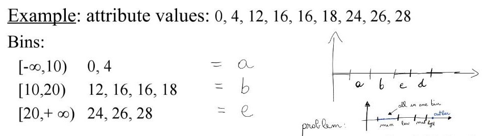
Discretization: converting quantitative variables into categorical variables by dividing the values in bins. Two simple discretization methods are equal width and equal depth.
- Equal-width: it divides the range into N intervals of equal size. The width of intervals will be W = (max - min)/N. It is sensitive to outliers; skewed data is not handled well, but it is the most straightforward.
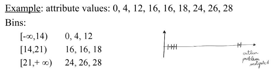
- Equal-depth: it divides the range into N intervals, each containing approximately the same number of samples. Good data scaling, minimizes information loss during the partitioning
- In both cases, the number of bins is defined by the user. Some rules of thumb:
- In case of classified data, it should not be smaller than the number of classes
- N_{bins} = \dfrac{M}{3 \cdot C}, where M is the number of training examples, C is the number of classes
One-Hot Encoding: convert a categorical variable to a numeric representation.
Complex data conversion procedures aim at building a small set of indices from a large number of variables, such that we reduce the number of features minimizing the information loss. Factor analysis and PCA are two statistical multivariate analysis techniques for data reduction.
Factor analysis identifies a group of shared underlying dimensions called factors. Each factor is a cluster of variables that correlate (positively or negatively) closely with one another. So, we compute the correlation of the variables, and we cluster them according to their correlation. Each cluster is a factor, and we can represent each factor with a new variable, thus reducing the number of variables. It is not a dependence method that designates specific variables as criteria with others as predictors. Instead, it is an interdependent approach where all variables are analyzed together, each interconnected with the rest.
Which value is assigned to the new variable? We take the linear combination of the variables in the cluster, weighted by their correlation, Y = w_1 X_1 + w_2 X_2 + ... + w_n X_n, where X_i are the variables in the cluster, and w_i are their weights (correlation values) called factor loading, the final value Y is called factor scores.
Output:
- Derived variables, generated records, and single-variable transformed data
3.4.4 Integrate Data
The integration task aims at combining information from multiple tables to create new records.
The result is the analytical data model, which represents a consolidated, integrated, and time-dependent restructuring of the data selected and preprocessed from the sources. In this task we define the unit of analysis, that is, the subject of the investigation, the major entity that is being analyzed in the study. The unit of analysis should not be confused with the unit of observation, which is the unit on which data are collected. For instance, a study may have a unit of observation at the individual level (e.g., pupils), but may have the unit of analysis at the level of a group (e.g., a class).
The unit of observation is the same as the unit of analysis when the generalizations being made from a statistical analysis are attributed to the unit of observation, that is, the objects about which data were collected and organized for statistical analysis.
The idea is that units of observation can be aggregated, while units of analysis cannot. For example, if we have data about individual customers (unit of observation), we can aggregate them to have data about households (unit of analysis). But if our unit of analysis is the household, we cannot disaggregate it to have data about individual customers. This common error is called the ecological fallacy, where inferences about individual behavior are drawn from data about aggregates.
If we want to draw conclusions about people, persons must be the unit of analysis. If we want to draw conclusions about households, households must be the unit of analysis.
So, integrating data means constructing the unit of analysis.
Output:
- Merged data which refers to joining two or more tables that contain different information about the same objects.
3.4.5 Format Data
Formatting covers syntactic modifications required by the modeling tool.
We format data in a common standard, like CSV, JSON, Parquet, etc.
Output:
- Reordered records, rearranged attributes
3.5 CRISP-DM: Modeling
3.5.1 Select Modeling Techniques
We need to select the modeling technique(s) that are appropriate to the data mining goals and the characteristics of the data.
We will choose on the basis of:
- The type of data mining task
- Ability to handle certain data types
- Ability to handle multiple relations and to generate relational patterns
- Explainability
- Scalability
- Level of familiarity
One can identify three primary components in any data mining algorithm:
- Model representation: relational vs propositional, quantitative vs qualitative, appropriateness for the intended user (human, computer, DM algorithm)
- Model representation is the language L used to describe discoverable patterns.
- Descriptive capacity:
- Quantitative discovery relates numeric fields (e.g., regression analysis)
- Qualitative discovery relates categorical fields (e.g., association rules, decision trees)
- Quantitative and qualitative discoveries are often expressed as simple rules. Putting together several simple implications, we obtain a logical theory that, under some assumptions, can be considered a causal theory.
- Descriptive capacity:
- Appropriateness: logic is more appropriate for the computer, natural language or visual depiction (like a decision tree) are more appropriate for humans.
- If the representation is too limited, then no amount of training examples or time will produce an accurate model for the data. A more powerful representation formalism increases the danger of overfitting; that is, a case in which the language of the model is not suited to that data (language bias, or induction bias).
- Model representation is the language L used to describe discoverable patterns.
- Model evaluation: estimates the uncertainty of a particular pattern. There are many ways to evaluate this uncertainty. Cross-validation is one of them.
- Search method: how to search the space of possible models, like greedy search, genetic algorithms, etc.
- We need to know whether search should be performed in the space of parameters, in the space of models (like the space of all decision trees, …) or both. For relatively simple problems there is no search: the optimal parameter estimates can be obtained in closed form. In general, a closed-form solution is not available. In this case, greedy iterative methods are commonly used (backpropagation).
Output:
- The modeling technique and any modeling assumptions of this technique (like probability distribution, no missing values, etc.)
3.5.2 Generate Test Design
Before building models, it is important to generate a procedure to test the quality of models.
Output:
- The test design, which describes the intended plan for training, testing and evaluating models.
3.5.3 Build Model
The model is applied to the data.
The output of a data mining algorithm can be expressed according to some industrial standards. The Predictive Model Markup Language (PMML) is an XML-based standard supported by many companies.
Output:
- Parameter settings and the rationale for their choice
- Output models together with expected accuracy, robustness, and possible shortcomings
3.5.4 Assess Model
Modeling results are interpreted according to data mining success criteria and the test design made before.
A model assessment should answer questions such as:
- How accurate is the model?
- How well the model describes the observed data?
- How much confidence can be placed in the model’s predictions?
- How comprehensible is the model?
3.5.4.1 Assessing descriptive models
A theoretical way to measure the expressiveness of rules is the minimum description length, that is, the number of bits it takes to encode both the rule and the list of all exceptions to the rule. The fewer bits required, the better the rule (Occam’s razor).
3.5.4.2 Assessing predictive Models
Predictive models are assessed on their accuracy on previously unseen data
- Model assessment can take place at the level of the whole model or at the level of individual predictions.
- Two models with the same overall accuracy may have quite different levels of variance among the individual predictions
- Model assessment should be based on a test set independent from the training set
- We need to evaluate the bias-variance tradeoff.
Output:
- Assessment of generated models
- Revision of parameter settings
3.6 CRISP-DM: Evaluation
3.6.1 Evaluate Results
This task evaluates models according to the KPIs defined in the business understanding phase. The challenge is to present new findings in a convincing, business-oriented way. This task is best done jointly by a data analyst and a business analyst.
Output:
- An overall assessment of data mining with respect to business success criteria (KPIs), including a final statement as to whether the project already meets the initial business objectives.
3.6.2 Review Process
The entire process is considered in order to determine if there is any important factor or task that is neglected or to identify a generic procedure to generate similar models in the future.
Output:
- Recommendation for further activities
The key question is:
“Have we found something that is interesting, valid and operational?”
Almost always the answer is no, in which case the exploratory cycle repeats itself, after having reviewed the process itself. The specific activities in this step depend on the kind of application that is being developed.
Common problems, for example in predictive models, are the failure to perform satisfactorily, overfitting, inability to generalize to new data, and problems in the collected data
3.7 CRISP-DM: Deployment
3.7.1 Plan Deployment
This task develops a strategy for deployment. In this phase we study the assimilation of knowledge, that is, formulate ways in which the new information can be best exploited, and how the final users must assimilate the capacity to use the new information given, or the new tool.
Output:
- A deployment plan
3.7.2 Plan Monitoring and Maintenance
Careful preparation for a maintenance strategy helps to avoid unnecessarily long periods of incorrect usage of data mining results.
Output:
- A maintenance plan for the monitoring process.
3.8 CRISP-DM: Produce Final Report
At the end of the project it is better to write up a final report, which can be a summary of the project, a final presentation of the data mining results, or both.
Output:
- A report or a final presentation or both
3.9 CRISP-DM: Review Project
Assess what went right and what went wrong, what was done well and what needs to be improved
Output:
- Experience documentation helps to consolidate important experiences made for future projects. The documentation may include pitfalls, misleading approaches, or hints for selecting the best-suited data mining technique in similar situations.
3.10 Summary Overview of CRISP-DM Phases
| Phase | Subphase | Description | Output |
|---|---|---|---|
| Business Understanding | Determine business objectives | Identify the primary goals from a business perspective. | Business objectives, business success criteria (KPIs). |
| Business Understanding | Assess situation | Consider resources, constraints, assumptions, and other factors that may influence project success. | Inventory of resources/constraints/assumptions, glossary of terminology, cost-benefit analysis. |
| Business Understanding | Determine data mining goals | Transform business objectives into technical data mining goals. | Data mining goals, success criteria for data mining goals. |
| Business Understanding | Produce project plan | Describe the plan for achieving data mining goals, including steps, duration, resources, inputs, outputs, and dependencies. | Project plan (e.g., Gantt chart). |
| Data Understanding | Collect initial data | Access relevant data from available sources, such as data warehouses. | Initial data collection report (data sources, collected data, problems encountered). |
| Data Understanding | Describe data | Examine data properties, including format, potential values, quantity, and field identities. | Data description report (format, potential values, quantity, field identities, surface information). |
| Data Understanding | Verify data quality | Inspect data for accuracy, completeness, consistency, and up-to-dateness. | Data quality report (findings, possible solutions if problems exist). |
| Data Understanding | Explore data | Combine statistical methods and visualizations to understand data content, distributions, and relationships. | Data exploration report. |
| Data Preparation | Select data | Choose relevant data based on goals, quality, and constraints; perform sampling and feature selection. | Rationale for inclusion/exclusion. |
| Data Preparation | Clean data | Address noise, outliers, and missing values to improve data quality. | Data cleaning report (decisions, actions, transformations, impacts). |
| Data Preparation | Construct data | Generate derived variables, new records, or transformed values; perform normalization, discretization, etc. | Derived variables, generated records, single-variable transformed data. |
| Data Preparation | Integrate data | Combine information from multiple sources to create the unit of analysis. | Merged data (joined tables, new values by summarizing). |
| Data Preparation | Format data | Apply syntactic modifications required by the modeling tool. | Reordered records, rearranged attributes. |
| Modeling | Select modeling techniques | Choose appropriate techniques based on task type, data characteristics, explainability, scalability, etc. | Modeling technique and assumptions. |
| Modeling | Generate test design | Create a procedure for training, testing, and evaluating models. | Test design (intended plan). |
| Modeling | Build model | Apply the algorithm to the data with optimal parameters. | Parameter settings with rationale, models with expected accuracy/robustness/shortcomings. |
| Modeling | Assess model | Interpret results according to success criteria; evaluate accuracy, robustness, comprehensibility, bias-variance tradeoff. | Assessment of models, revision of parameter settings. |
| Evaluation | Evaluate results | Assess models against business KPIs; present findings convincingly. | Overall assessment of data mining vs. business success criteria. |
| Evaluation | Review process | Identify neglected factors or generic procedures for similar projects. | Recommendations for further activities. |
| Deployment | Plan deployment | Develop strategy for exploiting knowledge and assimilating it by end-users. | Deployment plan. |
| Deployment | Plan monitoring and maintenance | Prepare strategy to monitor and maintain results. | Maintenance plan. |
| Deployment | Produce final report | Create summary report or presentation of the project and results. | Final report or presentation. |
| Deployment | Review project | Assess what went right/wrong and document experiences. | Experience documentation (pitfalls, hints). |