6 Apache Spark
Apache Spark is a cluster computing engine designed for big data and in-memory processing. It allows code and models to run in a distributed environment by following a programming paradigm called MapReduce.
MapReduce requires that the user writes two functions in the code:
- Map: takes as input a key-value pair and returns a set of intermediate key-value pairs.
- Reduce: takes as input an intermediate key-value pair (in which the value is a collection) generated by the Map, and generates new key-value pairs in which the initial values are merged into only one.
To work correctly, the reduce operation must apply a function that is both associative and commutative, because we don’t know in which order the reduce operations will be performed since they are executed in parallel.
Here is an example of an algorithm written with MapReduce:
Consider the problem of counting the number of occurrences of each word in a large collection of documents.
map(String key, String value):
    // key: document name
    // value: document contents
    for each word w in value:
        EmitIntermediate(w, "1");

reduce(String key, Iterator values):
    // key: a word
    // values: a list of counts
    int result = 0;
    for each v in values:
        result += ParseInt(v);
    Emit(key, result);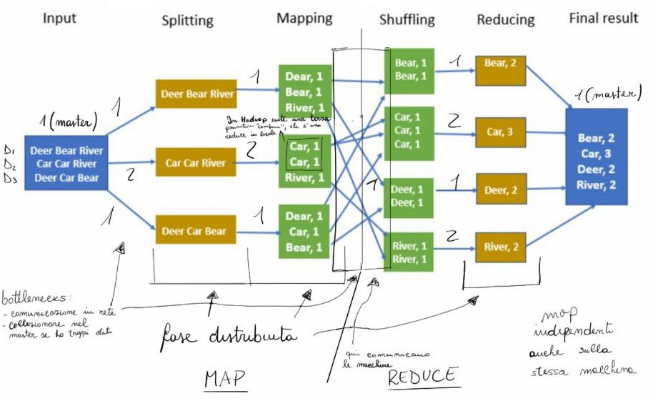
In the splitting phase, key-value pairs are created, one for each document, with the document content as the value. From this phase onwards, the algorithm becomes distributed, as each map computation for each document can be executed on multiple different devices. The map function is then applied to produce a set of key-value pairs representing the number of occurrences for each word in the given document. The shuffling phase groups the intermediate key-value pairs by key to create new key-value pairs in which the values are collections. These pairs are the input of the reduce function to reduce the collection values in each pair to a single value. Finally, all the pairs are aggregated and returned to the client.
Grouping pairs requires that the pairs to be grouped are on the same device. To achieve this, during the shuffling phase, devices communicate to have pairs with the same key on the same machine. This shuffling relies on a distributed file system shared among the different devices. This network communication is the main bottleneck of this framework. Another issue is that the final collection of all pairs will be stored on the master node. Furthermore, MapReduce works on secondary disk and requires numerous read and write operations. This problem is amplified when multiple MapReduce operations are chained sequentially.
Spark utilizes the MapReduce paradigm using distributed main memory managed by the master node, rather than relying on disk storage managed by individual devices. Spark also extends the MapReduce framework with additional functions like sample, join, etc. Spark supports streaming as an execution model. All these improvements significantly reduce the computation time.
The main Spark classes are: SparkContext (manages the entire distributed computation) and CassandraSQLContext (manages SQL operations on the distributed Cassandra database).
6.1 RDD & Operations
RDD (Resilient Distributed Dataset) is an object that is automatically distributed among the available devices. All key-value pairs handled during the computation are stored in an RDD. It handles the splitting phase automatically. Spark automatically handles node failures by redistributing the objects. RDDs are read-only (immutable). We can initialize an RDD from a file in the master’s memory, load it from an object in the SparkContext, or load a table from Cassandra.
The main types of operations on RDD are:
- Filter: returns a new RDD by applying a filter function to the input RDD.
- Distinct: returns a new RDD by removing duplicates from the input RDD.
- Join: given an RDD of key-value pairs, returns an RDD where values for matching keys are combined.
- Map (Map operation): given an RDD of key-value pairs, returns a new RDD of key-value pairs by applying a transformation function to each pair.
- FlatMap (Map operation): similar to map, but can map a single key-value pair to multiple key-value pairs.
- GroupByKey (Shuffle operation): given an RDD of key-value pairs, returns an RDD of key-value pairs where each value is a collection of all values for that key.
- ReduceByKey (Reduce operation): given an RDD of key-value pairs where values are collections, returns an RDD with key-value pairs where each value is a single aggregated value.
- Collect (Final aggregation): Returns a List object from the input RDD.
Broadcast variables: read-only variables shared across all devices, so everybody can read at the same time.
Accumulators: variables shared across all devices that can be used as accumulators. These variables can be written to by all workers, so everybody can write at the same time.
6.2 SparkSQL
SparkSQL is a Spark module for structured data processing that provides connectivity to databases and the possibility to execute SQL queries. It introduces two additional data types: DataFrame and Dataset. Both are handled as database tables, allowing us to execute queries on them.
Datasets are similar to DataFrames, but data within a Dataset are compressed using an Encoder in a format that allows Spark to perform operations like filtering, sorting and hashing without deserializing the bytes back into an object.
Additionally, Spark SQL can automatically infer the schema of a JSON dataset and load it as a DataFrame.
6.3 Spark MLLib
There are two main Spark libraries for machine learning: MLLib RDD-based and MLLib DF-based. The difference is that the former works with RDDs while the latter works with DataFrames.
MLLib introduces several new data types:
- Local Vector: represents a feature vector for dataset samples. A vector can be dense or sparse.
- Labeled Point: a pair (local vector, label)
- Local Matrix: represents matrices, which can be dense or sparse
LibSVM is a textual format used to represent datasets where each row represents a sample defined as “label index1:value1 index2:value2 …”. We can import a LibSVM dataset as an RDD of Labeled Points.
Note: if vectors or matrices are not wrapped in an RDD, they are not distributed. In general, you can create an RDD of matrices, but each individual matrix within the RDD is not itself distributed, the single matrix is considered as a unit, so the internal elements of the matrix are not distributed, every matrix is a monolithic unit. To distribute the elements of a matrix, specialized data types like RowMatrix are required.
The main ML models are implemented in MLLib, with some adaptations to work efficiently in a distributed environment (they must work using the MapReduce paradigm).
6.4 Spark Structured Streaming (2nd Generation)
A stream processing engine is in charge of sending data to the streaming application for processing. Even in the event of failure, a stream processing engine can offer three different sorts of assurances:
- At most once: data is delivered to an application no more than one time, but it could be zero time;
- At least once: data is delivered to an application one or more times;
- Exactly once: data is delivered to an application exactly one time.
Spark Structured Streaming provides fast, scalable, fault-tolerant, end-to-end exactly-once stream processing without requiring users to explicitly handle streaming semantics. Built on top of the Spark SQL engine, the key idea is to treat streaming computations like batch computations. The incoming data stream is conceptualized as a table, with new data arrivals represented as new rows being appended to the table.
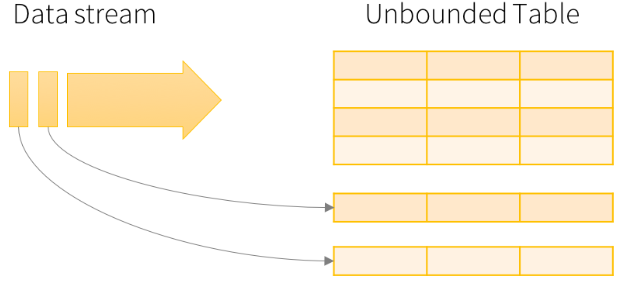
A stream of incoming data can be viewed as a table being continuously appended to, allowing existing structured APIs for DataFrames and Datasets (from SparkSQL) to be leveraged.
Spark Structured Streaming supports two execution modes:
- Continuous execution (or Record-at-a-time): the model immediately processes each piece of incoming piece of data as it arrives;
- Micro-batching: the model waits and accumulates a small batch of input data based on a configurable batching interval and processes each batch in parallel
Every Spark Structured Streaming application defines five core components:
- Data Source
- Programming Logic
- Output Mode
- Trigger Mode
- Data Sink
Structured Streaming provides native support for multiple data sources:
- Kafka Source: for reading from Apache Kafka
- File Source: supports different formats from various filesystems (HDFS, S3, etc.)
- Socket Source: for testing purposes only
- Rate Source: for testing purposes only; generates multiple events per second, each composed of a timestamp and a monotonically increasing value
Structured Streaming supports three different output modes:
- Append Mode: The default output mode. Only newly appended rows in the result table are sent to the output sink (existing rows are never overwritten).
- Complete Mode: The entire result table is written to the output sink.
- Update Mode: Only rows that have been updated in the result table are written to the output sink.
The Trigger information determine when to execute the provided streaming computation logic on the newly discovered streaming data. By default, Spark uses the micro-batch mode and processes the next batch of data as soon as the previous batch of data has completed processing. Alternatives are fixed interval, one-time and continuous processing.
Data sinks are the output destinations for streaming applications, used to store the results of stream processing:
- Kafka Sink: for writing to Apache Kafka
- File Sink: for writing to files
- Foreach Sink: for running custom computations on each output row
- Console Sink: for testing purposes only
- Memory Sink: for testing purposes only
6.5 Spark Structured Streaming & Spark MLlib
Applications combining streaming and machine learning can be divided into two parts:
- Batch Part: where the model is trained
- Streaming Part: where the model is applied to incoming test data streams
In the batch part of the application:
- Define a dataset schema to be used in the streaming part
- Read the training dataset
- Split the dataset into training and test sets
- Create a preprocessing pipeline
- Train the machine learning model
In the streaming part of the application:
- Evaluate the model on incoming data:
- Split the test data to simulate a data stream
- Read the simulated stream of test data
- Apply the preprocessing pipeline to the stream
- Generate and display predictions