5 Bayes Optimal Classifier and Ensemble Learning

Given instances X, training example D <x_i, c(x_i)> and target concept c, we want to determine a hypothesis h \in H such that h(x) = c(x) \forall x \in X. The learning task is to determine a hypothesis h identical to (which approximates) the target concept c over the entire set of instances X.

For simplicity, we assume that the hypotheses H are conjunctions of constraints on the attributes.

A hypothesis h covers a positive example if it correctly classifies the example as positive. An example satisfies h when h(x) = 1 regardless of whether x is a positive or negative example of c.

A hypothesis h is consistent with an example <x, c(x)> if h(x) = c(x). A hypothesis h is consistent with a training set D if it is consistent \forall x \in D.

Given two hypotheses h_k and h_j, h_j is more general or equal to h_k (h_j \geq h_k) iff any instance that satisfies h_k also satisfies h_j. h_j is strictly more general than h_k (h_j > h_k) iff h_j \geq h_k and h_k \not \geq h_j. The inverse relation (more specific than) can be defined as well.

The version space VS_{H, D} is the subset of hypotheses from H that are consistent with the training data D:

VS_{H, D} = \{ h \in H | Consistent(h,D) \}

The version space can be represented by its most general and least general members (version space representation theorem):

The general boundary G, with respect to hypothesis space H and training data D, is the set of maximally general members of H consistent with D:

G = \{ g \in H | Consistent(g, D) \land \neg \exists g^{'} \in H: g^{'} > g \land Consistent(g^{'}, D) \}

The specific boundary S, with respect to hypothesis space H and training data D, is the set of minimally general (maximally specific) members of H consistent with D:

S = \{ s \in H | Consistent(s, D) \land \neg \exists s^{'} \in H: s > s^{'} \land Consistent(s^{'}, D) \}

5.1 Bayesian Framework

Given the observed training data D we are interested in determining the best hypothesis from some space H. For classification tasks, the hypothesis is a classifier. What is the best hypothesis? It’s the most probable, given the data D plus any initial knowledge about the prior probabilities of the various hypotheses in H.

Bayes theorem provides a way to calculate the probability of a hypothesis based on prior probabilities + observed data.

P(i | h_1): probability that instance i is classified as positive by hypothesis h_1
P(i, h_1) = P(h_1) \cdot P(i | h_1): joint probability that hypothesis h_1 is correct and instance i is classified as positive by h_1
If we know the joint probability, P(X) = \sum_Y P(X, Y) (marginal probability)
Total probability: P(i) = \sum_{h_j \in H} P(i, h_j) = \sum_{h_j \in H} P(h_j) \cdot P(i | h_j)

Some notation:

h to indicate the hypothesis
P(h) the prior probability of h, that is, the initial probability that hypothesis h holds before observing the training data, reflecting the background knowledge we have.
P(D) the prior probability of the training data D, that is, the initial probability of observing the training data D before considering any hypothesis.
P(D | h) the likelihood of the data D given hypothesis h, that is, the probability of observing the training data D if we assume that hypothesis h holds.
P(h | D) the posterior probability of hypothesis h given the data D, that is, the probability that hypothesis h holds after observing the training data D.

Using Bayes theorem, we can express the posterior probability P(h | D) as:

P(h | D) = \frac{P(D | h) \cdot P(h)}{P(D)}

P(h | D) increases with P(h) and with P(D|h), and decreases as P(D) increases, because the more probable it is that D will be observed independent of h, the less evidence D provides in support of h. In other words, the support to the hypothesis h provided by the training data D is proportional to the likelihood P(D | h) and to the prior probability P(h) of the hypothesis, and inversely proportional to the prior probability P(D) of the training data.

The maximally probable hypothesis h \in H is the MAP hypothesis h_{MAP}:

h_{MAP} = argmax_{h \in H} P(h | D) = argmax_{h \in H} \frac{P(D | h) \cdot P(h)}{P(D)} = argmax_{h \in H} P(D | h) \cdot P(h)

We drop P(D) because it is constant for all hypotheses in H.

By assuming that all hypotheses are equally probable, the equation can be further simplified: the hypothesis that maximizes P(D|h) is the most probable. P(D|h) is called the likelihood of the data D given h.

The hypothesis P(D | h) is called a maximum likelihood hypothesis:

h_{ML} = argmax_{h \in H} P(D | h)

A maximum likelihood hypothesis does not incorporate any prior knowledge about the probability of the various hypotheses in H, because we are assuming that all hypotheses are equally probable.

The MAP hypothesis h_{MAP} incorporates prior knowledge about the hypotheses in H, because it takes into account the prior probabilities P(h) of the hypotheses.

5.1.1 Applying Bayes Theorem to Classification

X instance space
c: X \rightarrow {0, 1} the classification function to be learned
H hypothesis space
h \in H is a boolean function h: X \rightarrow {0, 1}, classifying instances as positive (1) or negative (0)

The goal is to find h such that h(x) = c(x) \forall x \in X.

Brute-Force MAP Learning Algorithm

Assumptions:

Deterministic and noisy-free data, that is, d_i = c(x_i) for all training examples <x_i, d_i>
c \in H (the representation language can “encode” the data)
All hypotheses h \in H are equally probable.

Given a training set D = \{<x_i, c(x_i)> | i = 1, ..., n\} of n training examples, where each example is an instance x_i \in X together with its classification c(x_i) \in {0, 1}, we want to find the most probable hypothesis h \in H given the training data D. For each hypothesis h \in H, we can compute the posterior probability P(h | D) using Bayes theorem and output the hypothesis h_{MAP} with the highest posterior probability.

To estimate P(h), for assumption (3) P(h_i) are all equal \forall h_i \in H and for assumption (2) \sum_{h_i \in H} P(h_i) = 1 so P(h_i) = \frac{1}{|H|} \forall h \in H. For assumption (1), P(D | h) = 1 if h is consistent with D, 0 otherwise. To estimate P(D) we use theorem of total probability + mutual exclusion of hypotheses:

P(D) = \sum_{h_i \in H} P(D | h_i) \cdot P(h_i) = \sum_{h_i \in VS_{H, D}} 1 \cdot \dfrac{1}{|H|} + \sum_{h_i \not \in {VS}_{H, D}} 0 \cdot \dfrac{1}{|H|} = \dfrac{|VS_{H, D}|}{|H|}

where VS_{H, D} is the subset of hypotheses from H that are consistent with D.

Therefore, when h is inconsistent with the training data D, P(h | D) = 0 \cdot \dfrac{P(h) }{P(D)} = 0, otherwise P(h | D) = \dfrac{1 \cdot \dfrac{1}{|H|}}{\dfrac{|VS_{H, D}|}{|H|}} = \dfrac{1}{|VS_{H, D}|}.

Under previous choices of P(h) and P(D | h), every consistent hypothesis has posterior probability equal to \dfrac{1}{|VS_{H, D}|}, and every inconsistent hypothesis has posterior probability 0.

Therefore, all consistent hypotheses are equally probable, and the MAP learning algorithm can return any consistent hypothesis (consistent learners).

The class of consistent learners is the class of learning algorithm that outputs a hypothesis that commits zero errors over training examples. Every consistent learner outputs a MAP hypothesis, under the assumptions previously made.

The Bayesian framework allows one way to interpret learning algorithms even when they do not explicitly manipulate probabilities, in Bayesian terms. In this way we can understand what assumptions the learning algorithm is implicitly making (inductive bias), we can compare different learning methods and analyze how well a learner generalizes based on its implied “probability model” of the world.

5.1.2 Bayes Optimal Classifier

So far we have considered the question:

What is the most probable hypothesis given the training data D?

Now we consider the question:

Given a new instance x, what is the most probable classification for x, given the training data D?

First solution: use the most probable hypothesis h_{MAP} to classify x, that is, output h_{MAP}(x). This is called the MAP classifier.

We can do better by combining the predictions of all hypotheses, weighted by their posterior probabilities. If the possible classification of the new example can take on any value v_j from some set V, then the probability P(v_j | D) that the correct classification for the new instance is v_j is just:

P(v_j | D) = \sum_{h_i \in H} P(v_j | h_i) \cdot P(h_i | D)

This principle is at the basis of any ensemble learning algorithm.

Any system that classifies new instances with the classification v_j that maximizes P(v_j | D) is called a Bayes optimal classifier:

v_{BO} = argmax_{v_j \in V} P(v_j | D) = argmax_{v_j \in V} \sum_{h_i \in H} P(v_j | h_i) \cdot P(h_i | D)

Formally, given the space hypothesis H and dataset D, we can demonstrate that no other classification method using the same hypothesis space and same prior knowledge can outperform the Bayes optimal classifier on average, in terms of expected classification error.

A curious property (shared then by ensemble methods) is that predictions it makes can correspond to a hypothesis not in H: the search space of Bayes Optimal Learner is not H, but H^{'}, which includes hypotheses that perform comparisons between linear combinations of predictions from multiple hypotheses in H.

The problem with this approach is that it is infeasible because we need to enumerate all the hypotheses in H, compute their posterior probabilities P(h_i | D) and their predictions P(v_j | h_i) for all possible classifications v_j \in V.

For this reason we can approximate P(v_j | D) \approx P(v_j | h_{MAP}) P(h_{MAP} | D). Since P(h_{MAP} | D) is constant for all classifications v_j \in V, the decision is actually based on the maximum value of P(v_j | h_{MAP}).

An alternative approximation is given by a randomly selected hypothesis. This leads to the Gibbs algorithm:

Choose a hypothesis h \in H at random, according to the posterior probability distribution over H.
Use h to predict the classification of the next instance x

The surprising finding is that the expected misclassification error of the Gibbs algorithm is at most twice the expected error of the Bayes optimal classifier:

E[error_{Gibbs}] \leq 2 \cdot E[error_{BayesOptimal}]

This means that:

We can pick any hypothesis from VS_{H, D} at random with uniform probability and the expected error is not worse than twice Bayes optimal.
We can pick several hypotheses from VS_{H, D} at random with uniform probability and the “ensembled” expected error is not worse than twice Bayes optimal (like picking randomly some trees from the space of possible trees in Random Forest).

In general, the performance of Bayes algorithm provides a natural standard against which other algorithms may be (theoretically) compared.

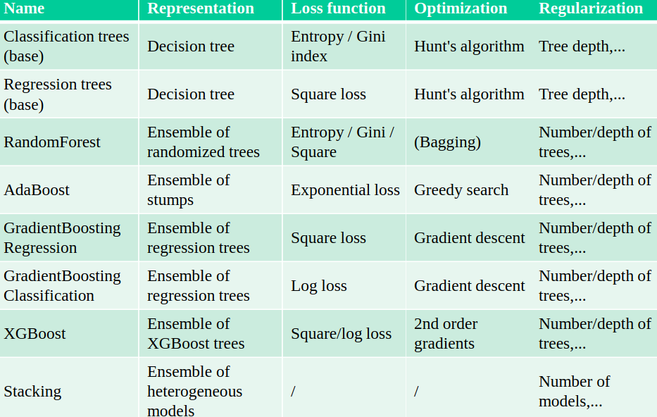
5.2 Ensemble Learning

Voting classifier: we simply average the predictions
- Hard voting: each classifier votes for a class and the class with the most votes is selected (class order breaks ties)
- Soft voting: each classifier outputs a probability for each class, and the class with the highest average probability is selected: argmax_c \sum_{m = 1}^{M} w_c p_{m ,c}, where p_{m, c} is the probability of class c predicted by classifier m and w_c is the weight of class c
- Classes can get different weights w_c

Why ensembling?

Different models may be good at different data split (even if they underfit)
Individual mistakes can be ‘averaged out’ (especially if models overfit)
With respect to the Bayes Optimal Classifier, we can now pick hypotheses from different spaces.

We choose the ensemble methods analyzing the bias-variance tradeoff¹:

If model underfits (high bias, low variance) we combine with other low-variance models: every model is an ‘expert’ on different parts of the data.
- We aim to reduce bias without increasing variance too much. Can be done with Boosting
If model overfits (low bias, high variance) we combine with other low-bias models: individual mistakes need to be different.
- We aim to reduce variance without increasing bias too much. Can be done with Bagging

Models must be uncorrelated but good enough.

We can also learn how to combine the predictions of different models, using a Stacking approach.

5.2.1 Bagging

Bagging (Bootstrap Aggregating) generates different models by training the same base model on different bootstrap samples of the training data. This reduces overfitting by averaging individual predictions, primarily decreasing variance while keeping bias relatively unchanged.

In practice, we create I bootstrap samples from the original dataset and train a separate model on each. A higher I leads to smoother predictions but increases computational cost for training and inference. Oversmoothing can slightly increase bias, but otherwise, bias remains largely unaffected.

Predictions are made by averaging the outputs of the base models: for classification, this often involves soft voting, and for regression, taking the mean value.

Additionally, bagging can provide uncertainty estimates by combining the class probabilities (or variances in regression) from individual models.

Given an ensemble trained for I iterations, it is possible to add more models later. However, this is less ideal if data batches change over time (concept drift), where boosting is more robust.

5.2.1.1 Random Forest

An example of bagging is the Random Forest algorithm, which builds multiple decision trees on bootstrap samples of the data. It introduces further randomness by selecting a random subset of features for each split in the trees, decorrelating the trees. A variant is Extremely Randomized Trees (Extra Trees), which considers a random threshold for a random subset of features at each split.

Random Forests do not require cross-validation; instead, it uses out-of-bag (OOB) error for evaluation. Since each tree is trained on a bootstrap sample, approximately 1/3 of the data is left out. These OOB samples can estimate model performance without a separate validation set, speeding up model selection (though the estimate is slightly pessimistic). Random Forests also provide reliable feature importance scores, derived from many alternative tree hypotheses.

Pros of Random Forest are that they don’t require a lot of tuning, are typically very accurate, handle heterogeneous features well, and implicitly select most relevant features.

Cons are that Random Forest are less interpretable and slower to train, and don’t work well on high dimensional sparse data (text).

5.2.2 Boosting

5.2.2.1 AdaBoost

Adaptive Boosting (AdaBoost) combines multiple weak classifiers to create a strong classifier. It works by iteratively training weak classifiers on the training data, with each iteration focusing more on the instances that were misclassified by previous classifiers.

Base models should be simple so that different instance weights lead to different models. We can train underfitting models called Decision stumps, very simple models, like pattern rules or very shallow trees.

AdaBoost is an additive model: predictions at iteration I are the sum of base model predictions, and the models get a unique weight w_i:

f_I(x) = \sum_{i = 1}^{I} w_i h_i(x)

where h_i(x) is the prediction of the i-th weak classifier. AdaBoost minimizes an exponential loss. For instance-weighted error \epsilon:

\mathbf{L}_{exp} = \sum_{i = 1}^{n} e^{\epsilon(f_I(x))}

By deriving \dfrac{\partial \mathbf{L}}{\partial w_i} we can compute the optimal weight for each weak classifier as

w_i = \dfrac{1}{2} \ln\left(\dfrac{1 - \epsilon_i}{\epsilon_i}\right)

where \epsilon_i is the weighted error rate of the i-th weak classifier. This is the inverse function of the sigmoid function: the sigmoid function squashes values from (−\infty, +\infty) to (0, 1), in this way we are doing the contrary, we take the error rate in a probability form and we encode it outside the (0, 1) range.

Algorithm

Input:

D: training dataset
I: number of iterations
\lambda: learning rate (shrinkage parameter)

Steps:

Initialize sample weights: s_{n,0} \leftarrow \dfrac{1}{N} for all n = 1, ..., N
For each iteration i = 1, ..., I:
1. Build a decision stump using sample weights s_{n,i-1}
2. Compute weighted error rate: \epsilon_i \leftarrow \sum_{n: \text{misclassified}} s_{n,i-1}
3. Compute model weight: w_i \leftarrow \lambda \cdot \log\left(\dfrac{1 - \epsilon_i}{\epsilon_i}\right)
4. Update sample weights for each sample n:
  - If misclassified: s_{n,i} \leftarrow s_{n,i-1} \cdot e^{w_i}
  - If correctly classified: s_{n,i} \leftarrow s_{n,i-1} \cdot e^{-w_i}
5. Normalize weights: s_{n,i} \leftarrow \dfrac{s_{n,i}}{\sum_j s_{j,i}}
Final prediction: f(x) \leftarrow \sum_{i=1}^{I} w_i \cdot h_i(x)

5.2.2.2 Gradient Boosting

Ensemble of models, each fixing the remaining mistakes of the previous ones. Each iteration, the task is to predict the residual error of the ensemble.

This is an additive model, too: predictions at iteration I are the sum of base model predictions:

f_I(x) = g_0(x) + \sum_{i = 1}^{I} \mu \cdot g_i(x) = f_{I-1}(x) + \mu \cdot g_I(x)

where g_0(x) is the initial model, g_i(x) tries to estimate the residuals of the previous model f_{i-1}(x), and \mu is the learning rate.

The pseudo-residuals r_i are computed according to a loss function (e.g. least squares loss for regression and log loss for classification).

Base models should have low variance, but flexible enough to predict residuals accurately.

Gradient Boosting is very effective at reducing bias error. Boosting too much will eventually increase variance.

For regression:

Least squares loss: r_i = y_i - f_{I-1}(x_i)
Pseudo residuals: the prediction errors for every sample: r_i = y_i - \hat{y_i}
Initial model g_0 simply predicts y
For iteration m = 1, …, M:
- For all samples i=1…n, compute pseudo residuals r_i = y_i - \hat{y_i}
- Fit a new regression tree model g_m(x) to r_i
  - In g_m(x) each leaf predicts the mean of all its values
- Update ensemble predictions: \hat{y} = g_0(x) + \sum_{m = 1}^M \mu \cdot g_m(x)

For classification:

Binary log loss: \mathbf{L}_{log} = -\sum_{i=1}^{n} [y_i \log(p_i) + (1-y_i)\log(1-p_i)], where p_i is the predicted probability for sample i
Initial model g_0 predicts p = \log \dfrac{\# positive}{\# negative} (log-odds probability)
Pseudo-residuals (gradient of log loss): r_i = y_i - p_i
In g_m, each leaf predicts \dfrac{\sum_i r_i}{\sum_i p_i (1 - p_i)}

Gradient Boosting is typically better than random forests, but requires more tuning and longer training, but still does not work well on high-dimensional sparse data.

XGBoost is a faster version of gradient boosting that allows scalability: it doesn’t evaluate every split point, but only q quantiles per feature (binning). The gradient descent is sped up by using the second derivative of the loss function.

5.2.3 Stacking

We choose M different base models and generate the predictions. The stacker (meta-model) learns the mapping between predictions and correct label. This can also be repeated by multi-level stacking. Popular stackers are linear models (fast) and gradient boosting (accurate).

We can also do the cascade stacking: each model gets as input the original features + predictions of previous models.

Models need to be sufficiently different and be experts at different parts of the data.

Another variant of stacking is the multi-view learning, where we train different models on different feature subsets (views) of the data (but still on the same unit of analysis).

Bias error: systematic error, independent of the training sample; points can be predicted (equally) wrong every time. Variance error: error due to variability of the model with respect to the training sample; points are sometimes predicted accurately, sometimes inaccurately.↩︎