4 Variable Associations
In the field of descriptive data mining we aim to uncover interesting relationships and patterns among variables in a dataset.
Most of statistics is concerned with finding dependencies between variables. Therefore, statistics provide several tools for this descriptive task.
Methods can be distinguished on:
- The number of variables:
- Two (bivariate)
- Multiple (multivariate)
- The type of variables:
- Quantitative
- Qualitative (categorical)
| Number of Variables | Type of Variables | Technique |
|---|---|---|
| Bivariate | Quantitative | Pearson correlation coefficient, Spearman Rank Correlation Coefficient |
| Bivariate | Qualitative | Chi-square, Lambda, Spearman Rank Correlation Coefficient |
| Multivariate | Quantitative | Correlation matrix, Partial correlation matrix |
| Multivariate | Qualitative | Association rules (can be extended to mixed data) |
4.1 Bivariate Associations: Two Quantitative Variables
We use the Pearson correlation coefficient to measure the linear relationship between two quantitative variables X and Y.
Var(X) = E[(X - E[X])^2]
Var(Y) = E[(Y - E[Y])^2]
Cov(X, Y) = E[(X - E[X])(Y - E[Y])]
Var(X + Y) = Var(X) + Var(Y) + 2Cov(X, Y)
- Sample variance: measures variability in one variable X
S_X^2 = \frac{1}{n-1} \sum_{i=1}^{n} (x_i - \bar{x})^2
- Sample covariance: measures how two variables, X and Y, vary together
S_{XY} = \frac{1}{n-1} \sum_{i=1}^{n} (x_i - \bar{x})(y_i - \bar{y})
The Pearson correlation coefficient r is defined as:
r = \frac{Cov(X, Y)}{\sqrt{Var(X) Var(Y)}}
The sample version is:
r = \frac{S_{XY}}{\sqrt{S_X^2 S_Y^2}}
The value of r ranges from -1 to 1, where:
- r = 1 indicates a perfect positive linear relationship
- r = -1 indicates a perfect negative linear relationship
- r = 0 indicates no linear relationship
A linear relationship is a synonym of redundancy: when X increases, Y increases as well. A negative linear relationship indicates that when X increases, Y decreases.
Geometrically, the Pearson correlation coefficient represents the cosine of the angle between the centered data vectors of X and Y in a n-dimensional space. Centered means that we subtract the mean from each value, so the vectors originate from the origin.
The limitation of this method is that it only captures linear relationships.
4.2 Multivariate Associations: Multiple Quantitative Variables
When there are n numeric variables X_1, X_2, ..., X_n, we can compute the correlation matrix. It is a symmetric n x n matrix where the entry at row i and column j is the Pearson correlation coefficient between variables X_i and X_j. The diagonal entries are all 1, as each variable is perfectly correlated with itself.
The correlation matrix must be correctly interpreted: given that we are using Pearson correlation coefficients, the matrix captures only linear relationships between variables, isolating each pair of variables without considering the influence of others. In fact, we can have transitive correlations: if X_1 is correlated with X_2, and X_2 is correlated with X_3, it does not imply that X_1 is correlated with X_3.
To get a correct view of the phenomenon, it is necessary to use the partial correlation, that measures the degree of association between X_i and X_j after removing the linear effects of the other variables. This helps to isolate the direct relationship between the two variables of interest.
The formula for calculating partial correlation between X and Y, after removing effects of Z is:
r_{XY.Z} = \frac{r_{XY} - r_{XZ} r_{YZ}}{\sqrt{(1 - r_{XZ}^2)(1 - r_{YZ}^2)}}
- r_{XY} is the Pearson correlation coefficient between X and Y
- r_{XZ} is the Pearson correlation coefficient between X and Z
- r_{YZ} is the Pearson correlation coefficient between Y and Z
The situation can be depicted by a graph:
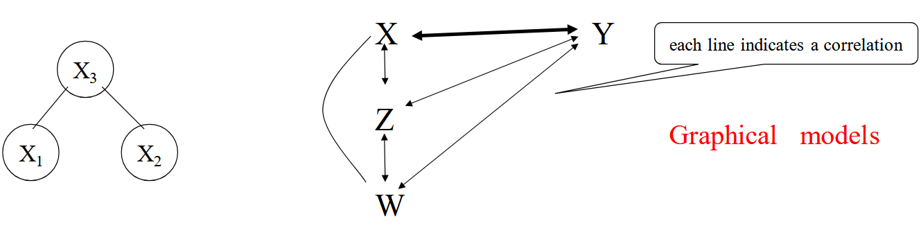
- X_1 and X_2 are correlated only through X_3
- They are uncorrelated when the effect of X_3 is removed
Under the assumption of Gaussian distribution for the variables:
- r_{XY} = 0 implies independence between X and Y
- r_{XY.Z} = 0 implies conditional independence between X and Y given Z
Graphical models investigate the use of graphs to express the conditional independencies between variables.
Generalizing, the computation of the partial correlation coefficient r_{12.j,j+1,...,n} between X_1 and X_2, controlling for all other variables X_j, ..., X_n, is recursive:
r_{12.j,j+1,...,n} = \frac{r_{12.j+1,...,n} - r_{1j.j+1,...,n} r_{2j.j+1,...,n}}{\sqrt{(1 - r_{1j.j+1,...,n}^2)(1 - r_{2j.j+1,...,n}^2)}}
where the base of recursion is given by r_{12}.
Therefore, to compute the partial correlation matrix we will compute all the partial correlations between each pair of variables, controlling for all other variables in the dataset. This matrix provides a more accurate representation of the direct relationships between variables, as it accounts for the influence of other variables. The result does not change if we change the order of the variables. I need to compute all the partial correlations because there is no monotonicity: for example, r_{12.3} can be significant, while r_{12.34} is not, it is not guaranteed that if we control for more variables the correlation decreases.
In a linear regression if we take X as independent variable and Y as dependent variable and we normalize them, then we obtain that
Y_{norm} = r_{XY} X_{norm}
In multiple regression models Y = \beta_0 + \beta_1 X_1 + \beta_2 X_2 + ... + \beta_n X_n + \epsilon regression coefficients \beta_i are related to partial correlation. In particular, in the case of variables standardized to unit variance (but not normalized) \beta_i = r_{y_i.1,2,...,i-1,i+1,...,n}.
4.3 Bivariate Associations: Two Qualitative (Categorical) Variables
It is not possible to measure association using Pearson. We need to use association measures: these measures quantify the strength and direction of the relationship between two categorical variables. They use frequency counts of occurrences of different combinations of categories from the two variables.
A typical association measure is the Chi-square, based on the null hypothesis of independence: there is no association between the two categorical variables.
\chi^2 = \sum_{i=1}^{r} \dfrac{(f_o^i - f_e^i)^2}{f_e^i}
- f_o^i is the observed frequency for category i
- f_e^i is the expected frequency for category i under the null hypothesis of independence: f_e^i = \dfrac{(row\ total)(column\ total)}{grand\ total}
- row total is the sum along i-th row, column total is the sum along i-th column, grand total is the sum of all frequencies of the entire frequency matrix
- The expected frequencies are calculated based on the assumption that the distribution of one variable does not depend on the other.
- r is the number of categories
If \chi^2 = 0, then there is no difference between observed and expected frequencies, so the two variables are independent (we accept the null hypothesis). The higher the value of \chi^2, the stronger the association between the two variables (we reject the null hypothesis).
Chi-square is a symmetric measure (\chi^2(X, Y) = \chi^2(Y, X)).
An asymmetric measure is Lambda. It measures the percentage of improvement in our ability to predict the value of the dependent variable once we know the value of the independent variable. This is based on the assumption that the best strategy for prediction is to select the value with most cases, since this will minimize the number of wrong guesses:
\lambda(y | x) = \dfrac{\sum_x max_y f_{xy} - max_y f_{.y}}{N - max_y f_{.y}}
- f_{xy} is the frequency count for category x of variable X and category y of variable Y
- \sum_x max_y f_{xy} is the majority voting knowing X
- max_y f_{.y} is the majority voting without knowing X
- N is the number of samples
We can also use a different heuristic than majority voting, even use a classifier.
The maximum value of \lambda(y | x) is 1, which occurs when prediction can be made without error, that is, when each independent variable value is associated with a single value of the dependent variable. A value of zero means no improvement in prediction.
- \lambda(y | x) = 1: I have all the info in X to predict Y
- \lambda(y | x) = 0: knowing X does not help to predict Y
Example: In a university course students are asked to rate the teaching staff. The univariate distribution for this variable looks like this:
| Rating | Frequency |
|---|---|
| Poor | 38 |
| Satisfactory | 32 |
| Good | 25 |
| Total | 95 |
Suppose you want to guess what the rating of another 95 people would be. Your best guess would be to pick the modal category, which is “Poor”. In this case you expect 38 right guesses and 57 wrong (out of 95 total guesses).
Now, suppose that you are given one additional piece of information. You now know what the ratings of the teaching staff are by the students in one of four years course.
| Rating | Freshman | Sophomore | Junior | Senior |
|---|---|---|---|---|
| Poor | 10 | 15 | 5 | 8 |
| Satisfactory | 5 | 10 | 15 | 2 |
| Good | 15 | 5 | 5 | 0 |
| Total | 30 | 30 | 25 | 10 |
Now, if you had to guess the teaching staff rating, you could qualify your best guess by knowing the year of student enrollment. For each year, you would guess the modal category:
| Year | Modal Category | Right Guesses | Wrong Guesses |
|---|---|---|---|
| Freshman (N=30) | “Good” | 15 | 15 |
| Sophomore (N=30) | “Poor” | 15 | 15 |
| Junior (N=25) | “Satisfactory” | 15 | 10 |
| Senior (N=10) | “Poor” | 8 | 2 |
| Total | 53 | 42 |
To compute Lambda explicitly:
Without knowing the year (univariate mode): Modal rating is “Poor” with frequency 38. So, right guesses = 38, wrong guesses = 95 - 38 = 57.
With knowing the year: For each year, predict the modal rating within that year:
- Freshman: Max frequency is Good (15), so right = 15, wrong = 30 - 15 = 15.
- Sophomore: Max is Poor (15), right = 15, wrong = 30 - 15 = 15.
- Junior: Max is Satisfactory (15), right = 15, wrong = 25 - 15 = 10.
- Senior: Max is Poor (8), right = 8, wrong = 10 - 8 = 2.
- Total right guesses knowing year: 15 + 15 + 15 + 8 = 53.
- Total wrong guesses knowing year: 15 + 15 + 10 + 2 = 42.
Lambda formula: \lambda = \frac{\sum_x \max_y f_{xy} - \max_y f_{.y}}{N - \max_y f_{.y}} = \frac{53 - 38}{95 - 38} = \frac{15}{57} \approx 0.263.
Note that (53-38)=(95-38)-(95-53)=(57-42)=15, that is, the number of new errors can be subtracted from the number of original errors and then divided by the number of original errors. This is an alternative formulation.
By knowing the year of student enrollment, we can reduce the error in predicting how they rate the teaching staff by 26.3%. This indicates a weak association between year of student enrollment and perception of the teaching staff.
Another way to measure association between two categorical variables is the Spearman Rank Correlation Coefficient. This is an index of correlation between two rank-order variables, that is, ordinal variables. It is defined as follows:
r_s = 1 - \dfrac{6 \sum d_i^2}{n(n^2 - 1)}
where D_i is the difference between ranks and n is the number of observations evaluated.
This association measure ranges between -1 and 1.
The SRCC can be shown to be equal to the Pearson correlation coefficient computed on the ranks of the data rather than the raw data values. This offers an alternative way to compute it:
- Sort X and Y
- Replace data with ranks
- Compute Pearson correlation coefficient on ranks
Example:
| x | y | x* | y* | |
|---|---|---|---|---|
| 0.1 | 0.4 | 1 | 1 | |
| 0.3 | 0.6 | 2 | 3 | |
| 0.5 | 0.5 | 3 | 2 | |
| 0.6 | 0.9 | 4 | 4 | |
| 0.8 | 1.8 | 5 | 6 | |
| 1.0 | 1.2 | 6 | 5 |
r_{pearson}(x, y) = 0.79 r_{spearman}(x*, y*) = 0.89
Association measures presented so far can be extended to accommodate multiple independent variables. Current practice appears to favor the use of log-linear models, but they are not so interpretable, and they are computationally heavy. To overcome these issues, we introduce association rules.
4.4 Association Rules
Association rules discovery is a descriptive data mining task. It aims at discovering relationships among items in a database.
Let’s introduce some notions. We will work on a database of transactions (tuples), where each transaction is a set of items (the columns in a tuple) to find frequent associations among sets of items in transaction databases.
Example:
| TID | Items |
|---|---|
| 1 | {A, B, C, D} |
| 2 | {B, C, E} |
| 3 | {A, B, D, E} |
| 4 | {A, C, D, E} |
| 5 | {B, D, E} |
| 6 | {A, B, C, E} |
A, B, C, D, E could be like “eggs”, “milk”, “bread”, “diapers”, “beer”. When we have quantitative attributes we can discretize the quantitative attributes to find association rules.
We want to find regularities in database of transactions. We can define two kind of regularities:
- “In 2% of transactions, customer purchase diapers, baby food, and beer together”: this is called support.
- “diapers” = yes AND “baby food” = yes AND “beer” = yes
- “In 70% of transactions where customer purchase diapers and baby food, they also purchase beer”: this is called confidence.
- “diapers” = yes AND “baby food” = yes => “beer” = yes
- This is an association rule.
An association rule is an implication of the form: X => Y, where X and Y are disjoint itemsets (sets of items). X is the antecedent, Y is the consequent.
More in general, we present an association rule with two measures s% and c%:
- s% is the support of the rule: percentage of transactions that contain both X and Y p(X \cup Y)
- c% is the confidence of the rule: percentage of transactions that contain X and Y among those that contain X p(Y | X), that is, the probability of buying the items in Y knowing that the items in X are bought.
To have business value a rule must have both support and confidence greater than some user-specified minimum thresholds. Low support OR low confidence means a useless rule.
We want to find an algorithm to do association rule mining that find all rules that correlate the presence of one set of items with that of another set of items that have support and confidence greater than user-specified minimum support and minimum confidence. So, given the ‘all’ in the previous sentence, every algorithm that works will find the same rules.
We can decompose the problem in two steps:
- Find the frequent itemsets: the set of items that have minimum support
- Use the frequent itemsets to generate association rules that have minimum confidence
- This is done in the same way for all algorithms:
- For each frequent itemset X
- For each proper nonempty subset A of X,
- Let B = X - A
- A \Rightarrow B is an association rule if confidence(A \Rightarrow B) = \geq min confidence, where support(A \Rightarrow B) = support(AB) and confidence(A \Rightarrow B) = support(AB) / support(A)
- For each proper nonempty subset A of X,
- For each frequent itemset X
- This is done in the same way for all algorithms:
Before introducing the algorithm, let’s consider a way to find the frequent itemsets with an example.
| TID | Items |
|---|---|
| 1 | {A, B, C} |
| 2 | {A, C} |
| 3 | {A, D} |
| 4 | {B, E, F} |
We first check itemsets with length 1:
- A: 3/4 = 75% support (> min support)
- B: 2/4 = 50% support (= min support)
- C: 2/4 = 50% support (= min support)
- D: 1/4 = 25% support (< min support)
- E: 1/4 = 25% support (< min support)
- F: 1/4 = 25% support (< min support)
So, we keep {A}, {B}, {C}.
At the second step, we generate itemsets with length 2:
- {A, B}: 1/4 = 25% support (< min support)
- {A, C}: 2/4 = 50% support (= min support)
- {B, C}: 1/4 = 25% support (< min support)
Do we need to consider {A, D}, {B, E}, {B, F}, {E, F}? No, because the support follows the antimonotonicity property: P({A, B}) \leq P({A}) and P({A, B}) \leq P({B}). Therefore, if an itemset is infrequent, all its supersets are infrequent as well.
Here, reported in other words:
By definition, if an itemset I does not satisfy the minimum support threshold, min_sup, then I is not frequent, that is, P(I) < min_sup. If an item A is added to the itemset I, then the resulting itemset (i.e., I \cup A) cannot occur more frequently than I. Therefore, I \cup A is not frequent either, that is, P(I \cup A) < min_sup. This property belongs to a special category of properties called antimonotonicity in the sense that if a set cannot pass a test, all of its supersets will fail the same test as well.
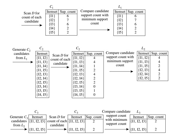
4.4.1 APriori Algorithm
- Input: transaction database, minimum support threshold
- Output: set of frequent itemsets with support \geq min support
Algorithm:
- Self-join step: Join the patterns L_{k-1} with itself to generate the candidate of length k C_k.
- Assume items in each itemset are sorted in lexicographic order (e.g., for a (k-1)-itemset l_i, l_i[1] < l_i[2] < \dots < l_i[k-1]).
- Two (k-1)-itemsets l_1 and l_2 are joinable if their first (k-2) items are identical: (l_1[1] = l_2[1]) \land (l_1[2] = l_2[2]) \land \dots \land (l_1[k-2] = l_2[k-2]) \land (l_1[k-1] < l_2[k-1]).
- The resulting k-itemset is \{l_1[1], l_1[2], \dots, l_1[k-2], l_1[k-1], l_2[k-1]\}.
- This ensures no duplicates and generates all possible candidates.
- Prune step: Remove candidates from C_k that have any (k-1)-subset not in L_{k-1}.
- Problem: scanning the database for all candidates in C_k can be computationally expensive if C_k is large.
- Solution: use the antimonotonicity property
- Thus, prune any candidate in C_k that has a (k-1)-subset not in L_{k-1}.
- This subset testing can be efficiently performed using a hash tree of frequent itemsets.
The drawbacks are that we need to scan the database multiple times and the number of candidates can be very large. The computational complexity is exponential in the length of the strings (Tartaglia’s triangle).
4.4.2 FP-Growth Algorithm
FPGrowth uses the Apriori pruning principle but scans the DB only twice, once to find frequent 1-itemsets, and once to construct the FP-tree (Frequent-Pattern tree), the data structure of FPGrowth.
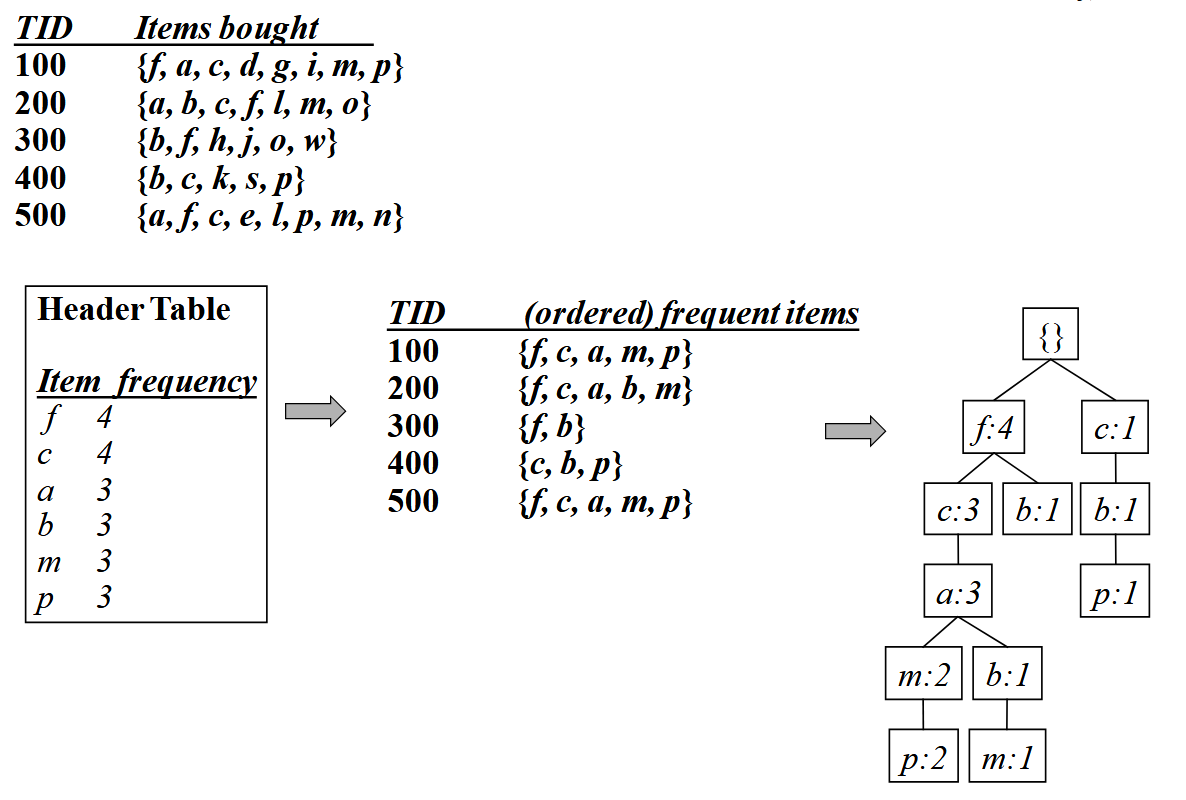
The Frequent Pattern Tree (FP-tree) is a compact data structure designed to store transaction information for frequent pattern mining. It consists of a null root node, a set of item-prefix subtrees representing transaction data, and a header table that provides direct access to all nodes for a given item. Each node in the tree contains the item’s name, a count of how many transactions share that path, and a link to the next node with the same item name, forming item-specific linked lists.
Constructing the FP-tree is a two-step process. First, the database is scanned once to identify all frequent items and their support counts. These items are then sorted in descending order of support. Second, the database is scanned again. For each transaction, its frequent items are sorted according to the header table and then inserted into the tree. During insertion, the algorithm traverses the tree, incrementing node counts along a shared path. If a path doesn’t exist, new nodes are created.
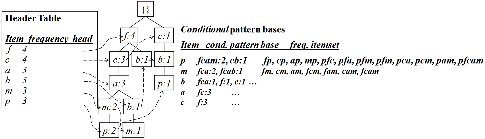
Frequent patterns are extracted from the tree using the FP-Growth algorithm, which employs a divide-and-conquer strategy. The algorithm recursively processes the tree to find patterns. For each frequent item, it generates a “conditional pattern base”, that is, the set of paths in the tree that end with that item. From this base, it builds a smaller, “conditional FP-tree” and mines it recursively. This process continues until the remaining tree has only a single path. At that point, all combinations of the items on that path are generated as frequent patterns, with their support being the minimum count of any item in the combination.