9 Machine Learning
Deduction is the core of expert systems. Now we will introduce an inductive approach, that is, machine learning.
What are the problems of Decision Support Systems? We have the Knowledge Acquisition Bottleneck:
- Experts not willing to elicit their knowledge
- Experts unable to formalize their knowledge
- Experts ignore details of their knowledge
The solution is to learn from data. In this way, we have a more comfortable, cheaper way to acquire knowledge automatically instead of encoding it manually.
The core of the learning is finding the same situation so we capture its relevance. Experience may modify the status of an organism in such a way that the new status makes the system capable of working better in a next situation.
Why are we in the induction setting? Because we start from facts to find general rules. The goal is to formulate general laws of the world starting from partial observations of the world itself.
Formally, given a set F of facts, and possibly, a set of inference rules having general validity, we want to find an inductive hypothesis that is true for all facts F and is true in the future for all and only those facts that are similar to those in F.
9.1 Formal definition of Machine Learning
A program learns from experience E with respect to a given set of tasks T and with a performance measure P if its performance on tasks T, measured through P, improves with experience E. Any learning program must identify and define the class of tasks, the performance measure to improve, and the source of experience.
9.1.1 Model of Machine Learning System in AI
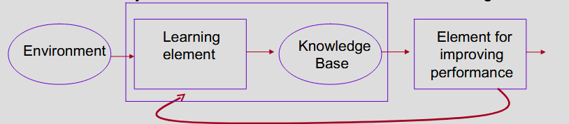
- Environment provides information to the Learning element, that uses it to improve the base of explicit knowledge
- Knowledge base expresses explicit knowledge in declarative form
- Performance element uses the knowledge to carry out its task at best. Additionally, the information acquired in the various attempts to carry out the task is used as feedback to the learning element
9.1.2 Types of Guidance
Now, some definitions:
- Observation: description of an object or situation in a given formalism
- Example: class label associated to an observation
For example, if I describe a chair or I have its properties, this is an observation. The moment I put the label “chair” to the observation, this is an example.
The unsupervised learning is based on observations, the supervised learning is based on examples, the semi-supervised learning is based on both observations and examples, the reinforcement learning is based on examples and feedback in response to the choices made, and the active semi-supervised learning is based on observations labeled interactively with an “oracle” (another model or other stuff).
- Relevance: components of the observations of interest for a given goal.
- Direct: explicitly indicated by the trainer (knowledge engineer/expert) for a specific observation
- Indirect: must be selected by the learner from the set of components associated with all available observations
9.1.3 Types of Objective
Objective can be:
- Predictive (Supervised): identify a relationship between a set of predictive variables and a target variable.
- Descriptive (Unsupervised): identify a relationship between a set of predictive variables and a target variable, but the target variable is not known. The best model may not be the most predictive one.
9.1.4 Representation
What are the questions needed to devise a suitable description?
- Is a set of object attributes (feature vectors, attribute-value pairs) sufficient for the learning task? Or are there relationships among objects?
- Which features do we need?
- Can the inductive assertion (concept) be expressed as the value of an attribute, as a predicate or as the argument of a predicate?
We have two kinds of representation:
- Sub-symbolic representation (unconscious reasoning): this is the mathematical/statistical approach. Examples: NN, clustering
- Symbolic representation (conscious reasoning, “perfect” explainability): this is the logical approach. Examples: Decision Trees, Classification Rules
There are several formalisms, synthesized in 2 large categories:
- 0-order learning (propositional logics), based on feature vectors or attribute-value pairs
- Example of feature vector: [shape, color, size, area] -> [triangular, red, medium, 0.75]
- Example of (Attribute-Value) pair: (shape = triangular) \land (size = medium) \land (color = red) \land (area=0.75)
- 1-order learning (predicate logics), based on complex schemes and allows relationships
To represent the acquired knowledge many “symbolic” learning systems express output as conjunctive concepts, like:
\phi = [color = red] \land [shape = square \lor triangle]
This can be also represented by a decision tree, for example.
9.1.5 0-Order learning
Input: vector or (attribute, value) pairs
Output: like the one seen before. Propositional calculus is sufficient to represent descriptions that are combinations of values of the attributes.
Now we consider the geometric representation of the input space. The input space is a multi-dimensional space where each dimension corresponds to an attribute. The points in the space are the observations. The goal is to find a hyperplane that separates the points of different classes.
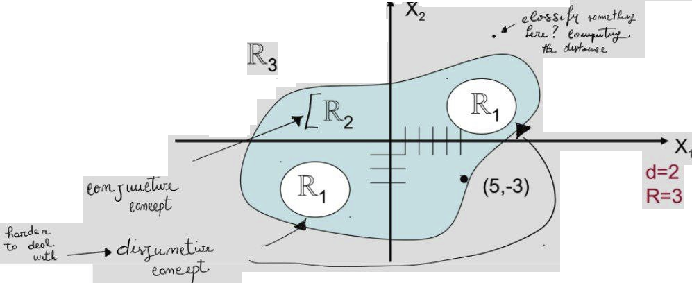
A classifier’s decision surfaces are implicitly defined by a set of discriminative functions g_1(X), g_2(X), ..., g_R(X), where X is the input pattern and R is the number of classes.
These functions are chosen such that:
For every input X \in \mathbb{R}^n, the classifier assigns it to class i if:
g_i(X) > g_j(X) \quad \text{for all } j \neq i
That is, the class corresponding to the maximum discriminative function value is selected.
This defines regions \mathbb{R}_i in the input space, where each region corresponds to inputs for which the i-th function is dominant.
Example (binary case, R = 2):
- Decide class c if g_1(X) > g_2(X)
- Otherwise, assign the alternative class.
These discriminative functions are required to be continuous, which ensures that decision surfaces are also continuous and well-defined.
9.1.6 1-Order Learning
It uses First-Order Logics and allows for a variable number of objects, relationships among them, and Inductive Logic Programming.
The input is an instance made of parts, attributes, relationships.
For example: e_1 = square(a) \land triangle(b) \land red(a) \land blue(b) \land on(b, a)
the output is an hypothesis defined in first order calculus:
\phi = red(Y) \land triangle(T) \land square(X) \land on(Y, X)
9.1.7 Conceptual Inductive Learning
The goal of Machine Learning is to satisfy the understandability postulate: the results of computer-made inductions should be symbolic descriptions of entities that are structurally and semantically similar to those that a human would produce. The components of such descriptions should be understandable as single information units.
It exploits a logic-like description language for inputs and outputs and different systems to represent experience and background knowledge to assess classification rules that define class patterns.
It allows conceptual descriptions of patterns that are similar to those that human experts would make when observing the same data.
A concept is an abstract description of a class. It is abstract because the name doesn’t matter (“mela” and “apple” are the same concept).
- Formation of concepts: grouping of instances in a set of classes (clustering)
- Attainment of concepts: search for defining attributes that distinguish instances of different classes.
Formation is the first step to Attainment.
9.1.8 Ensemble Learning
Learning of many models from one dataset. The final classification is a combination of predictions of the learned models. An example is random forest.
9.1.9 Deep learning
Multi-level learning, where we have a depth > 1 in the hierarchy of concepts. We learn hierarchically organized concepts where higher-level concepts are defined in terms of lower-level ones.
9.1.10 Lazy learning (or instance-based learning)
k-Nearest Neighbors.
9.1.11 Batch vs Incremental learning
- Batch: all observations/examples available at the beginning of the learning process. The assumption is that nothing more can happen outside the data, so if a new observation is added, we have to retrain the model from scratch
- Incremental: new observations/examples may become available subsequently
We need to have cooperation between the two approaches, in this way:
- Collect observations at the beginning
- Do batch learning
- If a new observation arises: fix the model incrementally
- At any moment (rarely) retrain from scratch
A system can be closed-loop: a learning system that can take the learned knowledge as an input to another learning process. Otherwise, it is an Open-loop system.
Batch learning uses a scanning strategy, which is a horizontal technique, comparing examples to find differences, while incremental learning uses focusing, which is vertical on the single example.
9.1.12 Stages of Learning
- Training: the system learns from examples
- Testing: the system is tested on a set of examples
- Tuning (in incremental approaches): refine the model when a new example arises.
9.1.13 Partitioning of Examples
- Training set, used in batch approaches
- Test set, used to evaluate the performance of the model after training
- Tuning set, used in incremental approaches
- Validation set, aimed at searching the best parameters for the learning algorithm
9.1.14 General definition of a model
Given:
- A language for describing examples
- A language for describing concepts
- A set of positive and negative examples of the concept to learn
- A function that checks if an example belongs to a concepts (coverage)
- A background knowledge
Determine:
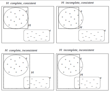
- An hypothesis in the hypothesis space that is consistent and complete (so correct) with respect to the examples and fulfills the constraints set on the background knowledge
Inductive inference requires the use of a matching procedure that may be based on a covering relation between a generalized description \phi and an instance f:
\phi covers f iff \phi(f) = true
It is a computationally feasible problem at the propositional level but NP-complete in first-order, because of the assignment of objects to variables.
A hypothesis h covers a positive instance x if it correctly classifies that example. An example satisfies a hypothesis if it is compliant with the conditions reported in the hypothesis, independently of its being labeled as a positive or negative example for the target concept.
A hypothesis is consistent with a set of training examples D iff h(x) = c(x) for each example (x, c(x)) \in D.
9.2 Inductive Learning as Search
- Search space = Hypotheses space (domain of the features) (nodes)
- Operators = Generalization rules + abduction + abstraction + … (arcs)
- Final state = One of the hypotheses that is consistent and complete with respect to the available observations.
But what is the “best” hypothesis? Since induction is a search in the space of descriptions, the goal of the search must be specified. In addition to completeness and consistency, descriptions are required to be discriminative and characterizing:
- Discriminative: defines all properties of the objects in that class necessary to distinguish them from objects in other classes
- Characterizing: defines facts and properties that are true for all objects in a class. How do we characterize? via Maximally Specific Characterization: the most detailed description that is true for all known objects belonging to the class.
9.3 Concept Learning
Concept learning is inferring a boolean-valued function from training examples of its input and output: given (P, N, C, L):
- P: set of positive examples of the target concept
- N: set of negative examples of the target concept
- C: set of concepts
- L: available language
We want to define a relationship r:
- acceptable iff definable in terms of C in L
- characteristic iff satisfied by positive examples
- discriminant iff not satisfied by any negative example
- admissible iff characteristic and discriminant
9.3.1 Learning Logic Formulas
Generality ordering: given hypothesis H and H^{\prime} with extensions e(H) and e(H^{\prime}), we say that H^{\prime} is more general than H iff e(H) \subseteq e(H^{\prime}).
For example, cube(X) \land red(X) is more specific than cube(X), cube(X) is more specific than cube(X) \lor pyramid(X).
For the intensional case with first-order languages, we cannot use implication directly, because finding \forall f_1 and f_2 if f_1 implies f_2 or if f_2 implies f_1 is undecidable. The solution is to relax the problem, leading to \theta-subsumption, but this is still NP-hard. Another solution is the \theta_{OI} subsumption, in which we add the requirement to not bind two variables on the same object. In this way, some computation becomes quadratic.
Now, to search for the best hypothesis in the space of hypotheses, we can leverage several exploration strategies:
- Bottom-up: initially select one or more examples, formulate a hypothesis covering them and then generalize (or sometimes specialize) it in order to explain the remaining examples
- Top-down: initially formulate a very general hypothesis and then specialize (or sometimes generalize) it in order to adapt it as much as possible to the observed data
How do we generalize? Dropping conditions (from cube(X) \land red(X) to cube(X)) or replacing with more general predicates derived from background knowledge (from cube(X) to geometricShape(X)).
How do we specialize? Adding conditions or replacing with more specific predicates.
When do we specialize? If negative examples are available, generalization on positive examples may yield too general concept descriptions that cover negative examples (over-generalization). In such a case, one may specialize.
How many hypotheses consistent with a given number of examples do we have? Consider a universe including \mu objects, a training set of m objects and k classes; the number of concepts consistent with the training set is k^{\mu - m}.
How to reduce the number of consistent hypothesis? We use the inductive bias: any reason to prefer one among different consistent hypotheses, for example preferring hypotheses with a short, simpler description (Occam’s razor).
9.4 Find-S algorithm
- Initialize h to the most specific hypothesis in H
- For each positive training instance x
- For each attribute constraint a_i, in h
- If the constraint a_i is satisfied by x
- Then do nothing
- Else replace a_i in h by the next more general constraint that is satisfied by x
- For each attribute constraint a_i, in h
- Output hypothesis h
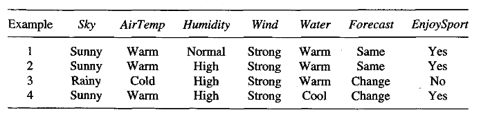
To illustrate this algorithm, assume the learner is given the sequence of training examples for the EnjoySport task. The first step of FIND-S is to initialize h to the most specific hypothesis in H (the first positive training example).
h \rightarrow (Sunny, Warm, Normal, Strong, Warm, Same)
Next, the second (positive) training example forces the algorithm to further generalize h, this time substituting a “?” in place of any attribute value in h that is not satisfied by the new example. The refined hypothesis in this case is
h \rightarrow (Sunny, Warm, ?, Strong, Warm, Same)
The FIND-S algorithm ignores every negative example: as long as we assume that the hypothesis space H contains a hypothesis that describes the true target concept c and that the training data contains no errors, then the current hypothesis h can never require a revision in response to a negative example. To complete our trace of FIND-S, the fourth (positive) example leads to
h \rightarrow (Sunny, Warm, ?, Strong, ?, ?)
The search moves from hypothesis to hypothesis, searching from the most specific to progressively more general hypotheses along one chain of the partial ordering.
9.5 Candidate-Elimination Algorithm
Intuition: start with an initial candidate Version Space (the subset of hypotheses from H consistent with the training examples in D) equivalent to the whole Hypotheses Space. Then use positive examples to remove too specific hypotheses (if any), and negative examples to remove too general hypotheses (if any).
How to do this?
- Start building a graph to represent the space of hypotheses that are consistent with the examples