7 Game Search in AI
7.1 Introduction to Multiagent Systems
In this chapter we examine multiagent systems, where multiple autonomous agents interact within a shared environment. Each agent attempts to solve its own task, possibly learning, while considering other agents’ actions.
7.2 Understanding Games in AI
7.2.1 Why Games Matter in AI Research
Games provide an ideal framework for studying intelligent decision-making for several reasons:
- Clear objectives: Success or failure is precisely measurable
- Controlled environments: Well-defined rules and boundaries
- Combinatorial complexity: Requires sophisticated knowledge representation and search strategies
- Learning opportunities: Provides feedback loops for improving strategies
7.2.2 Game Classification Framework
Games can be categorized along multiple dimensions:
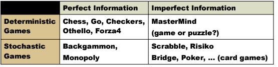
7.2.2.1 By Information Availability
- Perfect information games: All game states and actions are fully visible to all players (e.g., chess, tic-tac-toe)
- Imperfect information games: Some information is hidden from players (e.g., poker, battleship)
7.2.2.2 By Outcome Determination
- Deterministic games: Actions have predictable outcomes (e.g., chess)
- Stochastic games: Outcomes involve randomness (e.g., backgammon, poker)
7.2.2.3 Additional Classification Dimensions
- Number of participants: Single-player, two-player, or n-player games
- Turn structure: Sequential vs. simultaneous move games
- Environment type: Discrete vs. continuous state spaces
- Sum of outcomes: Zero-sum (one player’s gain equals another’s loss) vs. non-zero-sum games
7.3 Formalizing Games as Search Problems
Games can be transformed into structured search problems with these components:
- State space: The set of all possible game configurations
- Initial state: The starting configuration of the game
- Successor function: Rules defining legal moves and resulting states
- Terminal test: Determines when the game ends
- Utility function: Evaluates outcomes from a player’s perspective
For perfect information games, we can model the problem as a search tree where:
- Nodes: Represent game states
- Branches: Represent moves (actions) leading to new states
- Players: Two types alternate making decisions:
- MAX: Player trying to maximize utility (often “us”)
- MIN: Player trying to minimize utility (the opponent)
The tree structure alternates between levels where MAX decides and levels where MIN decides, with the goal of finding a path that maximizes utility assuming the opponent plays optimally.
7.4 The Minimax Algorithm
7.4.1 Core Concept
Minimax is a recursive decision algorithm designed for two-player zero-sum games with perfect information. It works by:
- Building a game tree to a certain depth
- Evaluating terminal positions
- Propagating values upward through the tree
- Selecting moves that maximize the minimum guaranteed outcome
The algorithm assumes both players play optimally - MAX tries to maximize the score while MIN tries to minimize it.
7.4.2 Mathematical Definition
Given a game tree, the Minimax value of a node n is defined as:
\text{Minimax}(n) = \begin{cases} \text{Utility}(n), & \text{if } n \text{ is a terminal state} \\ \max_{a \in Actions(n)} \text{Minimax}(Result(n, a)), & \text{if } n \text{ is a MAX node} \\ \min_{a \in Actions(n)} \text{Minimax}(Result(n, a)), & \text{if } n \text{ is a MIN node} \end{cases}
Where:
Actions(n): Returns all legal moves from statenResult(n, a): Returns the state resulting from actionaUtility(n): Evaluates the score of a terminal state
7.4.3 Implementation
7.4.3.1 General Algorithm
def minimax(state, depth, maximizingPlayer):
    if is_terminal(state) or depth == 0:
        return utility(state)

    if maximizingPlayer:
        value = float('-inf')
        for a in actions(state):
            value = max(value, minimax(result(state, a), depth - 1, False))
        return value
    else:
        value = float('inf')
        for a in actions(state):
            value = min(value, minimax(result(state, a), depth - 1, True))
        return value
7.4.3.2 Detailed Pseudocode with Path Tracking
MIN-MAX(Pos, Depth, Player)
    IF deep_enough(Pos, Depth) THEN  // Terminal or reached depth limit
        Value = static(Pos, Player)
        Path = NIL
    ELSE
        Successors = gen_move(Pos, Player)  // Generate possible moves

        IF Successors is empty THEN  // No moves available
            return Value = static(Pos, Player), Path = NIL
        ELSE  // Evaluate each possible move
            Best_value = minimum possible value for static()
            FOR Succ in Successors
                Succ_res = MIN-MAX(Succ, Depth + 1, opponent(Player))
                New_value = -value(Succ_res)  // Opponent's perspective
                IF New_value > Best_value THEN  // Found better move
                    Best_value = New_value
                    Best_path = Succ & path(Succ_res)
            return Value = Best_value, Path = Best_path
Where:
deep_enough(Pos, Depth): Returns TRUE if search should stop (depth limit or terminal state)gen_move(Pos, Player): Generates possible moves from the current positionstatic(Pos, Player): Evaluates position quality from Player’s perspectiveopponent(Player): Returns the opposing player
In practice, we use limited-depth search with a position evaluation function to handle complex games, evaluating non-terminal states to estimate their value.
7.4.4 Properties and Limitations
7.4.4.1 Theoretical Properties
- Completeness: Complete if the game tree is finite
- Time complexity: O(b^m), where b is the branching factor and m is maximum depth
- Space complexity: O(b \times m) using depth-first traversal
7.4.4.2 Practical Challenges
Non-quiescent states problem
Issue: Search cutoff might occur in volatile positions, leading to misleading evaluations
Solution: Quiescence search: continue searching in unstable positions beyond the normal depthHorizon effect
Issue: Algorithm may make poor choices that delay negative outcomes just beyond the search depth
Impact: Can lead to locally optimal but globally poor decisionsExponential complexity
Issue: Pure minimax becomes impractical for games with large branching factors
Solution: Apply pruning techniques to reduce the search space
7.5 Alpha-Beta Pruning
Alpha-Beta pruning is an optimization technique that dramatically reduces the number of nodes evaluated by the minimax algorithm without affecting the final result.
7.5.1 Key Insight
The key insight is that once we have found a move that proves a position is worse than a previously examined option, we can stop analyzing further moves from this position.
7.5.2 How It Works
- \alpha (alpha): Tracks the best value found so far for MAX along the path
- \beta (beta): Tracks the best value found so far for MIN along the path
The algorithm prunes branches when:
- At a MAX node: Current value \geq \beta (MIN will never allow this path)
- At a MIN node: Current value \leq \alpha (MAX has a better option elsewhere)
7.5.3 Efficiency Gains
The effectiveness of alpha-beta pruning depends on move ordering:
- With perfect move ordering: O(b^{(m/2)}) nodes evaluated vs. O(b^m) for plain minimax
- This effectively doubles the searchable depth, allowing the AI to look twice as far ahead
- The effective branching factor becomes \sqrt{b} instead of b
With these optimizations, games like chess, checkers, and Othello can be played by AI systems using minimax with alpha-beta pruning as their core strategy.