6  Search

6.1 Problem solving definition

Given:

• a (possibly partial) description of a current situation and of a desired situation.
• a list of operators that can be applied to situations to transform them into new situations.

Find a problem solution, that is, an operator in the process language that transforms the object describing the initial situation into the object describing the desired situation.

A state is a description of a situation, while the space of problem states is the set of all possible situations that the system can describe and distinguish. The problem space is a set of problem states along with a set of operators that can change the states.

Operators are functions that take a state and transform it into another. These are not applicable to any state but depend on the operator preconditions.

6.2 Choosing the Space of States

A state space is an abstraction of the real world, where states are sets of real states, and actions are complex combinations of real actions. A state space has the same set of possible real paths that are solutions in the real world. Obviously, each abstract solution should be simpler than in the real world.

Problems for which the algorithm is lacking are to be solved tentatively and must exploit a general search mechanism: the solution is to be searched in the space of possible problem states, and to reach a solution, it must allow choosing, at any moment, among the applicable operators, those that can be suitably applied to a state and transform it into a new state closer to the goal state. To do so, we use a Pattern-Directed Inference System.

6.3 Pattern-Directed Inference Systems

PDIS are programs that directly and dynamically respond to a range of not-known-in-advance data or events rather than working on expected data in a known format using a rigid strategy. Patterns are preconditions of operators.

PDIS has three components:

• A collection of modules, substructures that can be activated by patterns in the data.
• Working memory, one or more data structures that can be examined and modified by modules.
• An interpreter that controls the selection and activation of the modules.

6.4 Problem-Space Graph

A graph can be used to represent the space of a problem. The states are nodes, while operators are arcs. The state space is represented as a 4-tuple (N, A, S, G), where:

• N: set of states.
• A: set of operators.
• S: non-empty subset of N that includes the initial state.
• G: non-empty subset of N that includes the goal states.

A solution is a path in the graph, from an initial node in S to a node in G.

So the problem setup is:

• Define the “problem environment”: identify all possible configurations of the elements in the domain (state space) and distinguish legal or admissible states.
• Define the initial state.
• Define the goal states (also implicitly defining their properties).
• Define a set of operators, explicitly expressing the conditions that are to be satisfied in order to apply them.
• Generate a solution: search for those operators that allow reaching the goal states.

To model the solution process, we need to consider the representation of each node in the search process, the selection of applicable operators, the topology of the search process, and the possible use of local (in case of specific situations) or global (general) level knowledge to guide the search.

Control strategies may be used by the problem solver in the solution process. There are two approaches:

• Irrevocable: rules are chosen and never reconsidered. This is possible only when we have much knowledge (or an oracle), and it degrades to a deterministic search.
• Tentative: the chosen rules may be reconsidered to obtain better performance. This is needed when the deterministic solution is impractical. The solution is searched tentatively by trying to improve the efficiency of the procedure through a reduction of the search space using selective techniques (backtracking) or generative techniques (generate-and-test with greedy techniques).

Using backtracking, a search tree can be built. Every level in the tree is a stage in the solution. This is exhaustive, meaning it exploits the whole search space of the problem.

6.5 Backtracking strategy

A basic implementation can be the following:

function backtrack(Data):
    if term(Data):
        return []                   // Termination condition met
    if deadend(Data):
        return FAIL                 // Known dead-end

    Rules = applicable_rules(Data)  // Ordered list of applicable rules

    while Rules is not empty:
        r = first(Rules)            // Select first rule
        Rules = tail(Rules)         // Remove it from the list

        Rdata = r(Data)             // Apply rule to get new state
        Path = backtrack(Rdata)     // Recursive call on new state

        if Path != FAIL:
            return [r] + Path       // Prepend rule to the successful path

    return FAIL                     // No solution

1. term(.) predicate: true for arguments that satisfy the termination condition. If it terminates with success, the empty list is returned
2. deadend(.) predicate: true for arguments that are know not to belong to a solution path. In such a case, the procedure returns a failure
3. applicable_rules(.) predicate: function that computes the rules applicable to its argument, and orders them (arbitrarily or heuristically)
4. If there are no more rules to apply, the procedure fails.
5. Choose the best rule to apply
6. Reduces the list of applicable rules by removing the selected rule
7. Apply Rule R to produce a new DB
8. Recursively call the procedure on the new DB
9. If recursive call fails, try another loop
10. Otherwise add R to the list of successfully applied rules.

To avoid infinite loops during backtracking, we pass the list of visited database states (Dlist) as an argument, instead of the single state. This list:

• Records the path from the current state back to the initial state.
• Allows cycle detection by checking whether the current state has already been visited.
• Enforces a limit on search depth via a global BOUND value, helping prevent unbounded rule applications.

Details:

1. Dlist contains all database states visited in the current path, with the most recent state first.
2. The procedure fails if a state is revisited or the depth exceeds BOUND.
3. The current state is extended with each recursive call by adding the new state to the front of the list.

function backtrack(Dlist):
    Data = first(Dlist)

    if member(Data, tail(Dlist)): # tail(Dlist): written in Prolog style
        return FAIL  // Cycle detected

    if term(Data):
        return []  // Terminal state reached

    if deadend(Data):
        return FAIL  // No rules to apply

    if length(Dlist) > BOUND:
        return FAIL  // Search depth exceeded

    Rules = applicable_rules(Data)

    while Rules is not empty:
        r = first(Rules)
        Rules = tail(Rules)

        Rdata = r(Data)
        Rdlist = [Rdata] + Dlist  // Prepend new state to the visited path

        Path = backtrack(Rdlist)

        if Path != FAIL:
            return [r] + Path  // Prepend rule to the successful path

    return FAIL  // No valid path found

6.6 Search Strategies for Problem Solving

A graph may be explicitly specified (unfeasible in AI) or implemented dynamically, that is, generated during exploration. The control strategy itself makes explicit part of an implicitly specified graph. The solution path is built starting from an initial node n_0 and applying the set of rules that allow generating the nodes one after the other. Browsing the graph means building a new node by applying the successor operator to a node: expanding n_0, then the successor of n_0, and so on makes explicit a graph defined implicitly. The control strategy is the process to make explicit, through the generation of the search tree, a portion of an implicit graph that is sufficient to include a goal node.

A search algorithm is generally defined as follows:

1. Generate a search tree T_r consisting of only n_0. Add n_0 to an ordered list OPEN, including the nodes to be processed.
2. Generate a list CLOSED, initially empty.
3. If OPEN is empty, exit with FAILURE.
4. Choose the first node n in OPEN, extract it, and add it to CLOSED.
5. If n is the goal node, exit with SUCCESS with the solution obtained by backtracking from n to n_0.
6. Expand node n, generating a set M of successors. Add the nodes in M as successors of n in T_r, adding an arc from n to each element in M. Add these elements of M to OPEN.
7. Reorder the list OPEN based on some criterion. Here is where we use knowledge to make this search informative; otherwise, it is blind.
8. Go to step 3 until OPEN is empty.

This general search generates all successors of a node but can be modified to generate one successor at a time. Simply, the node is not put in CLOSED until all of its successors are generated.

It can be used to perform a search in different ways.

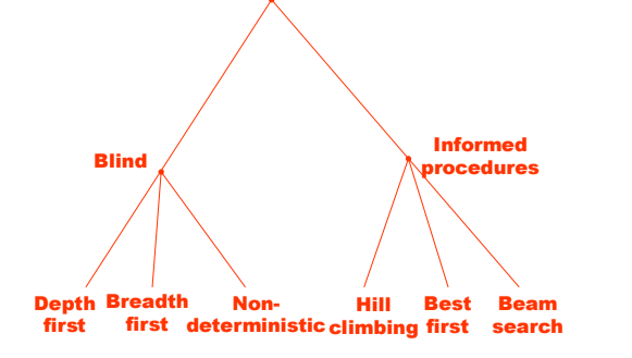
• Uninformed

• BFS: new nodes are added at the end of OPEN. Nodes in OPEN are ordered in descending order based on the depth of the search tree. Nodes at the same depth are arbitrarily ordered.

• DFS: new nodes are added at the beginning of OPEN. Nodes in OPEN are ordered in ascending order based on the depth of the search tree.

• Bidirectional Search: searching simultaneously both starting from the initial state toward the goal state, and from the goal state toward the initial state, letting the two borders meet in the middle. In general, if a DFS is used in one direction and a BFS in the other, their intersection is guaranteed.

• Informed

• Best first: new nodes are ordered using a local heuristic criterion. The procedure to search for a solution path may exploit local-level knowledge to choose the best rule to apply and generate the solution path with a good success probability.

• A*

6.6.1 A* Search

What if we want the best solution path? First of all, we define what “best” means. We can define a cost function that assigns a cost to each node in the search tree, and then we can use this cost function to guide our search. The cost function can be defined in different ways, depending on the problem domain and the specific requirements of the search. The aim is to minimize the cost of the path between two nodes, that is, find the best path between a given node s and another node t.

Let g(n) be the cost of the minimum cost path between the starting node s and node n, and h(n) be the cost of the minimum cost path between a node n and the goal node.

Ideally, we want to find a path from s to t with the minimum cost, that is, we want to minimize the cost function f(n) = g(n) + h(n).

For any node n, let us denote h^*(n) the heuristic factor, that is, the estimation of h(n), and g^*(n) the depth factor, that is, the cost of the lowest cost path found up to node n. A good search algorithm will use as an evaluation function f(n) = g^*(n) + h^*(n). The search algorithm will then select the node with the lowest value of f(n) to expand next.

An algorithm that uses this evaluation function is called A*:

1. Generate a search graph G consisting only of the starting node n_0. Add n_0 to an ordered list OPEN.
2. Generate a list CLOSED, initially empty.
3. If OPEN is empty, exit with FAILURE.
4. Choose the first node n in OPEN, extract it, and add it to CLOSED.
5. If n is a goal node, exit with SUCCESS with the solution obtained by tracing back the path along the pointers from n to n_0 in G.
6. Expand n by generating a set M of its successors that are not already ancestors of n in G. Add such elements of M in G as successors of n.
7. Generate a pointer to n from each element in M that is not already in G (i.e., in OPEN or CLOSED). Add such elements of M to OPEN. For all elements m in M that are already in OPEN or CLOSED, replace their pointer with one that points to n if the best path to m found so far is through n. For all elements in M already in CLOSED, change the pointer of each of its descendants in G so that they point back in correspondence to the best paths found so far for such descendants.
8. Sort list OPEN by ascending values of f^*. In case of ties on the minimum value of f^*, prefer the deepest node in the search tree.
9. GOTO 3.

A* is admissible, that is, it’s guaranteed to always find the optimum path if:

• Conditions on the graph: all nodes in the graph have a finite number of successors (if any), and all arcs in the graph have costs greater than or equal to a value \epsilon > 0.
• Condition on h^*: for all nodes n in the search graph, h^*(n) \leq h(n). This means that h^* never overestimates the real value h (optimistic estimation).

It is also complete, meaning it is guaranteed to find a solution if one exists.

The precision depends on the heuristic function. Given two versions A_1 and A_2 of A* with evaluation functions f_1(n) = g_1(n) + h_1(n) and f_2(n) = g_2(n) + h_2(n), with both h_1 and h_2 being lower bounds on h^*, we say that A_2 is more informed than A_1 if, for all non-goal nodes, h_2(n) > h_1(n). This means that A_2 is more precise than A_1 in estimating the cost of the path to the goal node.

6.6.2 Some notes about efficiency

Computational efficiency depends on the computational costs of the control strategy. There are two areas where we can optimize:

• The cost of applying the operators (processing a node in the graph) [cost of the heuristics].
• Control costs (reordering of the rules).

Typically, we have to find a trade-off between the two because they cannot be optimized simultaneously: if we have a lot of knowledge, then the control strategy is costly while the rule application cost is low because the system goes straight to the solution. On the other hand, with less knowledge, the rule application cost is high because many alternatives may be attempted.

6.6.3 Performance Measures

• Penetrance: P = \dfrac{L}{T}
  • L: length of the solution path found.
  • T: total number of nodes generated during the search.
  • Maximum value = 1, reached if the successor operator is precise.
  • Small values for blind search.
  • It measures how “elongated” the generated tree is.
• Branching value: \dfrac{B}{B-1} (B^L - 1) = T
  • B: constant number of successors each node should have in an imaginary tree of depth equal to the length of the path and with a total number of nodes equal to the number of nodes generated during the search.
  • We build a perfectly balanced tree of depth L, where each node has B successors.
  • If B is close to 1, then the search is focused toward the goal.
  • Penetrance can be expressed in terms of B: P = \dfrac{L}{T} = \dfrac{L(B-1)}{B (B^L - 1)}.